Rhodops is a progressively grown generative adversarial network (ProGAN) named after rhodopsin, a receptor protein found in the eye’s rods which is receptive to brightness. It was accepted to the gallery at the workshop on computer vision for fashion, art and design at ECCV 2018. You can view the rest of the accepted works in the online gallery.
Rhodops was trained on a dataset of images generated by multiple phases of style transfer. First, images were generated with 1 - 5 style images drawn randomly from a set of about 70 selected images. Once all the style images were represented in the set, generated images were fed back to the algorithm as content and style images. This process was repeated multiple times with different variations of drawing content and style images from each set until there were around 700 total generated images. These were enlarged, cropped in different places, rotated, inverted, and mirrored to create a larger dataset for the GAN to learn from.
Generating the Dataset
Style transfer was started at a resolution between 64x64 and 256x256 pixels (randomly chosen) and upscaled by a factor of the square root of 2 until 1024x1024. The histogram of the pastiche was matched to the style image at each scale. The starting size acts as a style-content tradeoff, starting larger will preserve the content more while starting smaller will increase the influence of the style on the final image. Each image took around 7 minutes to generate on a GTX 1080 Ti.
Random drawing of style images in the first stage is essentially an example of the coupon collector’s problem, styles are drawn until all the images have been collected. The expected amount of draws until all images have been drawn at least once can be approximated by n*log(n) + 0.577*n (where 0.577 is the Euler-Mascheroni constant). For 70 images this works out to about 170 draws. Upon visual inspection, a couple nice styles were still underrepresented so an extra 30 images were generated with combinations of those styles, leaving the first phase total image count at 200.
The next phase of style transfers randomly chose 1 of the generated images and styled it with 2 - 3 other images either from the original style set or the generated set. The idea was to make sure that certain shapes would be included in different styles so that the generator could perhaps learn to interpolate between styles for a given shape. Around 100 images were made in this way.
At this point most generated images were half black, half white by nature of random selection and the approximately even distribution of dark and light images in the original style set. To ensure that there would be more images that were majority black or majority white, dark and light images were separated into different sets. Now styles were drawn within the dark or light set, generating images that were majority dark or light. Some 250 images were generated in this way.
In the final phase, to foster the image set’s interrelatedness, 3 images were selected from the complete set and styled in a round robin. Each image was used as content with the other two as style.
Preparing data for the GAN
After 3 - 4 days of generating images the dataset was only 700 strong, clearly not enough to train a GAN with. To alleviate this, all the images were doubled in size using waifu2x and then cropped into overlapping tiles at different scales (e.g. 9 tiles of size 1448x1448 and 16 tiles of 1024x1024 from the full 2048x2048 image). Every tile was rotated 90, 180 and 270 degrees and tiles that were not on the edge of the full image were also rotated 45, 135, and 225 degrees. This turned every image into 136 new images ballooning the dataset to almost 100k images. ProGAN’s built in mirroring argument was enabled and a second inverting argument was added that inverted image’s colors, a final 4-fold increase.
Training
Finally ProGAN could be let loose on the dataset. Training took a week, however sadly on the final transition from 512x512 to 1024x1024 pixels the network suffered mode collapse. No amount of tweaking settings, retraining from checkpoints, or training on different datasets has been effective at avoiding collapse yet. This is an issue I’ve had when training on multiple different datasets. So far I’ve only reached 1024x1024 pixels once with a full color network, acryl. Mode collapse still gives some interesting results when interpolating though.
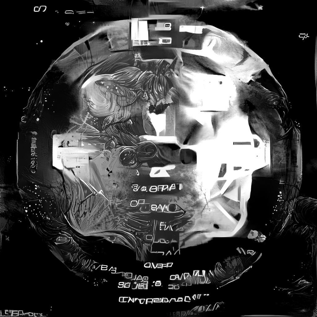
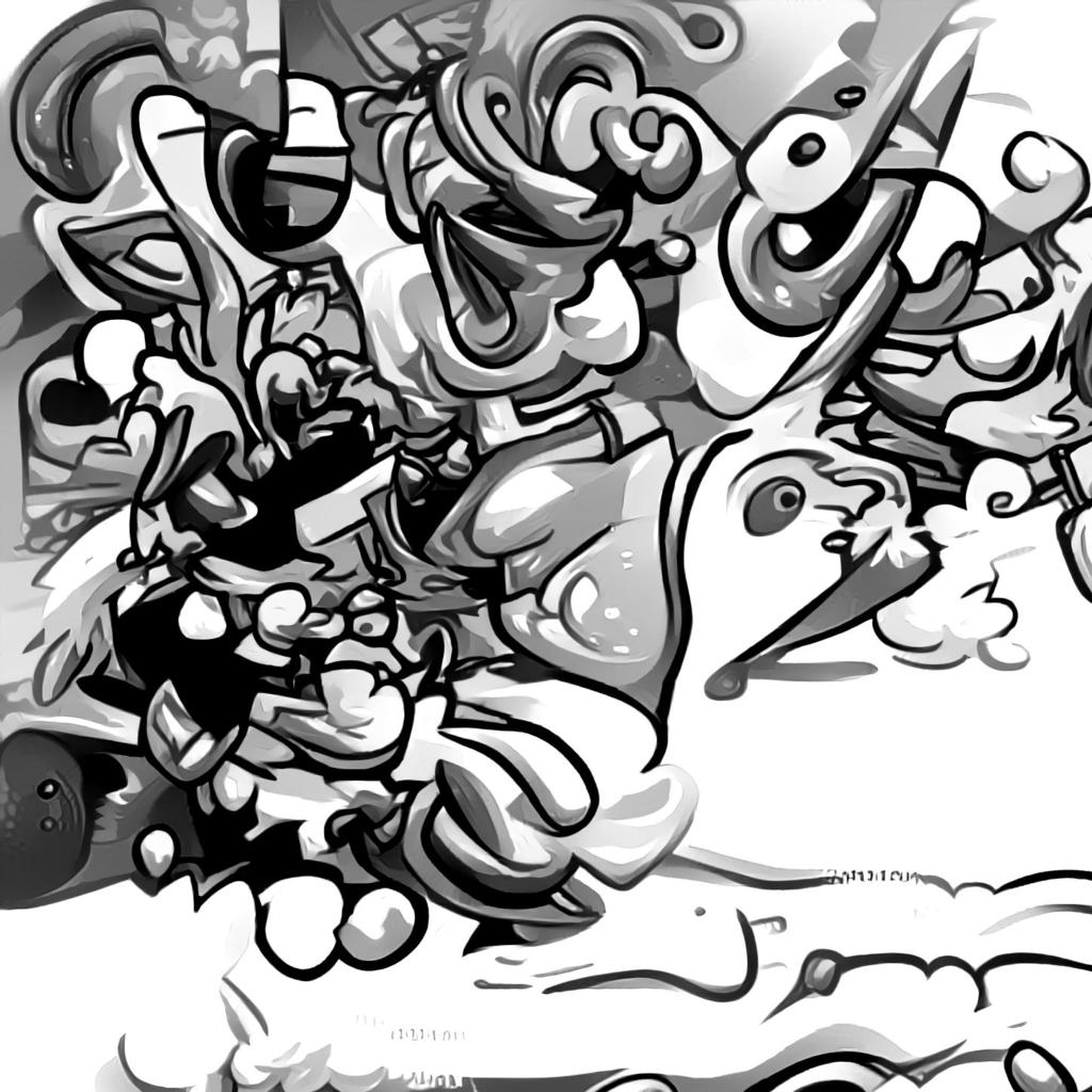
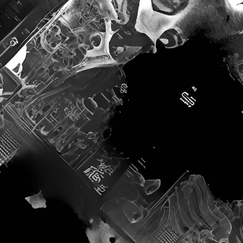
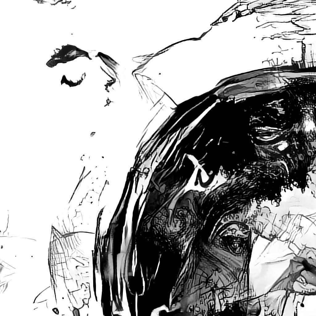
Anyways, mode collapse can’t ruin all the fun. A resolution of 512x512 is larger than anything DCGAN could generate and a lot of interesting details can already be seen.
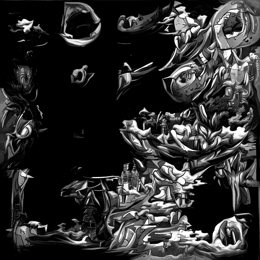
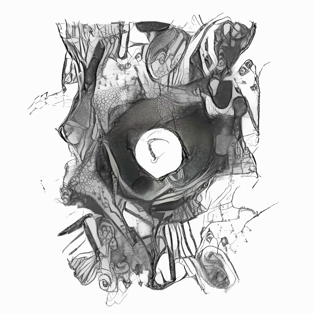
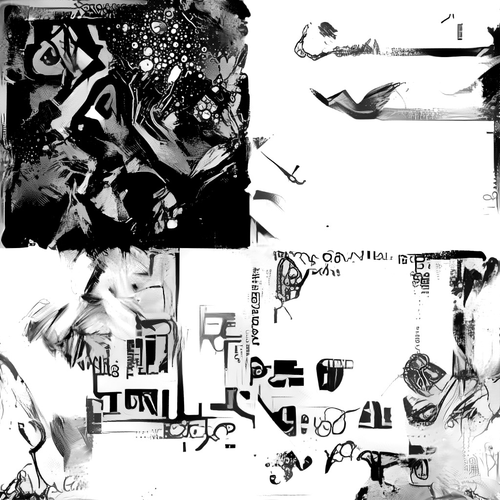
Results
MIDI Knob Control
Frame generation runs at around 15 frames per second so realtime interaction was an obvious next step. I hooked up each of the 8 knobs on my MIDI keyboard to 5 random values in the latent variable. 15 frames per second isn’t very nice to look at though (and often times a little jerky from the not so smooth MIDI knob operation), so the values of the latent variable are recorded throughout the session to be smoothed over and interpolated to higher frame rates afterwards.
Final Thoughts
All in all the results are pretty nice. While not all of the variation in generated input styles is captured by the GAN, it has an interesting interpretation of the dataset as a whole. Future projects will be to enhance the currently small resolution outputs with a pix2pix model and to hook the latent vector up to music frequency information for some automated music video generation.