In this post we give an overview of our replication of the paper Optimal Textures: Fast and Robust Texture Synthesis and Style Transfer through Optimal Transport for the Delft University of Technology Deep Learning course CS4240. First we’ll discuss the contributions in the paper as we understand them, then go over our implementation of each part, and finally compare the algorithm with competing techniques.
Our implementation in PyTorch, called optex, can be found here.
Overview
Optimal Textures presents a new approach for texture synthesis and several other related tasks. The algorithm can directly optimize the histograms of intermediate features of an image recognition model (VGG-19) to match the statistics of a target image. This avoids the costly backpropagation which is required by other approaches which try to instead match 2nd order statistics like the Gram matrix (the correlations between intermediate features). Compared to other algorithms which seek to speed up texture synthesis, Optimal Textures achieves a better quality in less time.
The approach builds on a VGG-19 autoencoder which is trained to invert internal features of a pretrained VGG-19 network back to an image. This was originally introduced by Li et al. in Universal Style Transfer via Feature Transforms. This autoencoder allows one to encode an image to feature space, perform a direct optimization on these features, and then decode back to an image.
The reason this approach is faster than the backpropagation-based approach is that the internal feature representation of the image is adjusted directly to make it more similar to the target. This allows the use of the decoder to get an optimized image back. With backpropagation, a loss is placed on the Gram matrices of the image and its targets. These correlations cannot be easily inverted back to the feature representation and so the decoder cannot be used. The image must then be updated based on the gradients calculated all the back and forth through the VGG network.
Algorithm
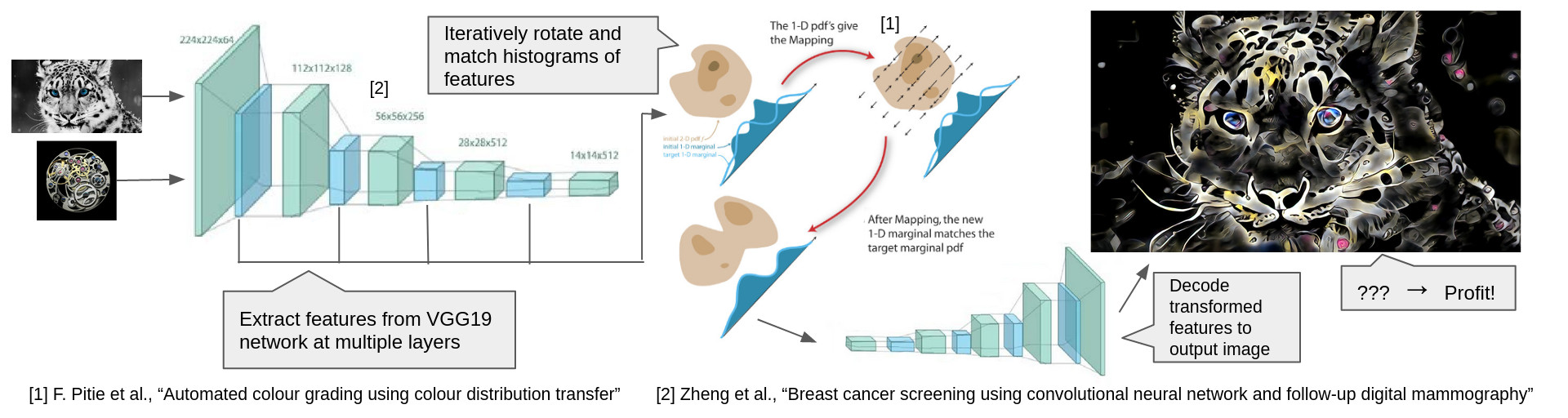
The core algorithm introduced by Optimal Textures consists of 4 steps:
- Encode a target and style image to the intermediate features of an image recognition network
- Apply a random rotation to the features of both images
- Match the histograms of the rotated feature tensors
- Undo the rotation and decode the features back to image space
Steps 2 and 3 are applied iteratively so that the histograms of the two images match from a large selection of random “viewing angles”. This process is also applied at 5 different layers within the VGG-19 network (relu1_1, relu2_1, relu3_1, etc.). This ensures that the statistics of the output image match the style image in terms of the entire hierarchy of image features that VGG-19 has learned to be important for distinguishing images.
Speeding things up
This relatively simple algorithm can be augmented by a couple techniques that improve the speed and quality of results.
The first technique is to project the matched features to a smaller subspace and perform the optimization there. The chosen subspace is the one spanned by the first principal components that capture 90% of the total variance in the style features. This reduces the dimension of the feature tensors while retaining the majority of their descriptive capacity.
The second technique is to synthesize images starting from a small resolution (256 pixels) and progressively upscaling during optimization to the desired size. Once again, this reduces the size of the feature tensors (this time along the spatial axes) which improves speed. Another benefit is that longer-range relations in the example image are captured as the relative receptive field of VGG-19’s convolutions is larger for the smaller starting images.
Extensions
The paper further shows how the basic algorithm can be used for multiple tasks similar to texture synthesis: style transfer, color transfer, texture mixing, and mask-guided synthesis.
Style transfer
To achieve style transfer, a content image’s features are added into the mix. The features of the deepest three layers of the output image are interpolated toward the features of the content image. Notably, the content image’s features must be centered around the mean of the style image’s features to ensure the two are not tugging the output image back and forth between distant parts of feature space.
Color transfer
The naive approach to color transfer would be to directly apply the optimal transport algorithm to the images themselves rather to their features. However, the paper introduces an extension of this which preserves the colors of the content image a little better. The basis for this technique is luminance transfer, which takes the hue and saturation channels of the content image (in HSL space) and substitutes them into the output of the optimal transport style transfer. The drawback of luminance transfer is that the finer colored details in the style are no longer present, but instead directly take the color of the underlying content. To remedy this, a few final iterations of the optimal transport algorithm are applied with the luminance transfered output as target. This gives a happy medium between the content focused color transfer of the luminance approach and the style focused color transfer of the naive optimal transfer approach.
Texture mixing
Another task which the paper applies the new algorithm to is texture mixing. Here, two styles should be blended into a texture which retains aspects of both. To achieve this, the target feature tensors are edited to have aspects of both styles. First the optimal transport mapping from the first style to the second and from the second style to the first is calculated. This is as simple as matching the histogram of each style with the histogram of the other as target. This gives 4 feature tensors that are combined to form the new target.
A blending value between 0 and 1 is introduced to control the weight of each style in the mixture. First each style is blended with its histogram matched version according to blending value. When the blend value is zero, the first style is unchanged, while the second style is 100% the version matched to the histogram of the first style. When the blend value is 0.75, the first style is 1/4 original, 3/4 histogram matched and the second style vice versa.
Next a binary mixing mask is introduced with the percentage of ones corresponding to the blending value. This mask is used to mix between the two interpolated style features. When the blend value is low, the majority of pixels in the feature tensor will be from the first style’s feature tensor, when it’s high the majority comes from the second style.
This is repeated at each depth in the VGG autoencoder. These doubly blended feature targets are then directly used in the rest of the optimization, which proceeds as usual.
Mask-guided synthesis
The final application of optimal textures is mask-guided synthesis. In this task, a style image, style mask, and content mask are used as input. The parts of the style image corresponding to each label in the style mask are then synthesized in the places where each label is present in the content mask.
To achieve this the histogram of the style features is separated into a histogram per label in the mask. Then the output images histogram targets in the optimization are weighted based on the labels in the content mask. Pixels which lie along borders between 2 class labels are optimized with an interpolation between the nearby labels based on the distance to pixels of that class. This ensures that regions along the borders interpolate smoothly following the statistical patterns present in the style image.
Replication
Now we will discuss our implementation of the above concepts. We’ve managed to replicate all of the above findings except for the mask-guided texture synthesis (partially due to time constraints, partially due to it not being amenable to our program’s structure).
Core algorithm
The core algorithm consists of only a few lines. We build upon one of the official repositories for Universal Style Transfer via Feature Trasforms. This contains the code and pre-trained checkpoints for the VGG autoencoder. This gives one PyTorch nn.Sequential module that can encode an image to a given layer (e.g. relu3_1) and a module that decodes those layer features back to an image.
One thing to note is that we follow pseudo-code from the paper which seems to invert the features all the way back to an image between each optimization at a given depth. It is also possible to step up only a single layer (e.g. from relu5_1 to relu4_1). This would improve memory usage significantly as a much smaller portion of the VGG network would be needed in memory. Right now memory spikes for the encode/decode operations are the limiting factor for the size which can be generated. Next to reducing memory this would also reduce FLOPs needed per encode/decode and so reduce execution time.
Once features are encoded, we need to rotate before matching their histograms. To this end, we draw random rotation matrices from the Special Orthogonal Group. These are matrices that can perform any N-dimensional rotation and have the handy property that their transpose is also their inverse. We’ve translated to PyTorch SciPy’s function that can draw uniformly from the N-dimensional special orthogonal group (giving us uniformly distributed random rotations). For each iteration, we draw a random matrix, rotate by multiplying both the style and output features by this matrix, perform histogram matching, and then rotate back by multiplying with the transpose of the rotation matrix.
Histogram matching
Matching N-channel histograms is the true heart of Optimal Textures. Therefore it is important that this part of the algorithm is fast and reliable. The classic way of matching histograms is to convert both histograms to CDFs and then use the source CDF as a look up table to remap each color intensity in the target CDF.

However, we found this method difficult to implement efficiently. First of all, the PyTorch function for calculating histograms, torch.histc, does not support batched calculation. Trying to use the (experimental as of time of writing) torch.vmap function to auto-vectorize also leads to errors (related to underlying ATen functions not having vectorization rules). Secondly, most implementations of this method we could find rely on the np.interp function which does not have a direct analogue in PyTorch. We tried translating the NumPy implementation to PyTorch, however, our implementation seems to create grainy artifacts for smaller number of bins in the histogram. Therefore we set the default to 256 instead of 128 as suggested in the paper.

As an alternative, we added the histogram matching strategies used by Gatys et al. in Controlling Perceptual Factors in Neural Style Transfer (our implementation is based on this implementation using NumPy). These strategies match histograms by applying a linear transform on different decomposition bases of the covariances of each histogram (principal components, Cholesky decomposition, or symmetric eigenvalues). These strategies can be applied directly to the entire encoded feature tensors (rather than channel by channel) and so are significantly faster. The decompositions all work on the covariance of the tensors which have shapes dependent on the number of channels. This side-steps the need for binned histograms as the covariances will have the same shape regardless of the input image dimensions.
Each basis gives slightly different results, although in general they are comparable to the slower CDF-based approach.

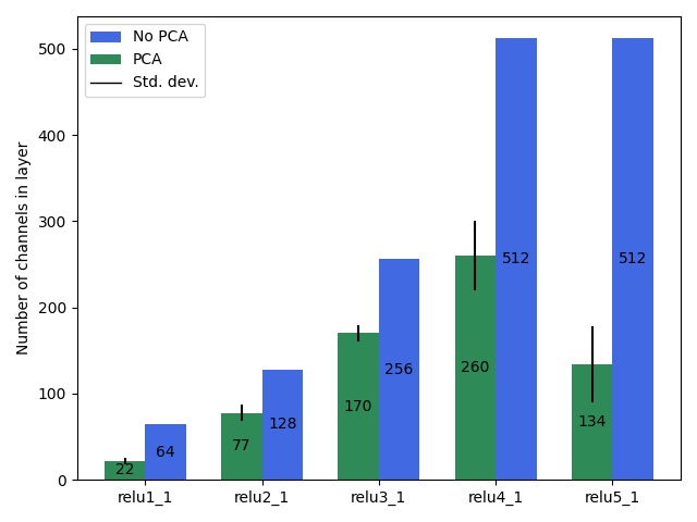
PCA
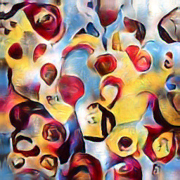
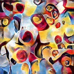
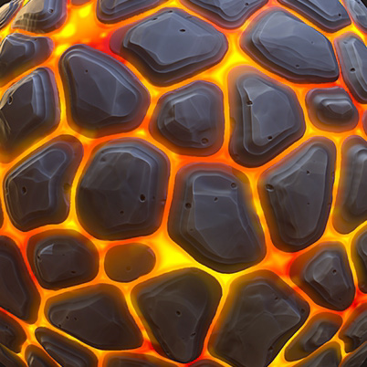
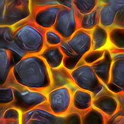
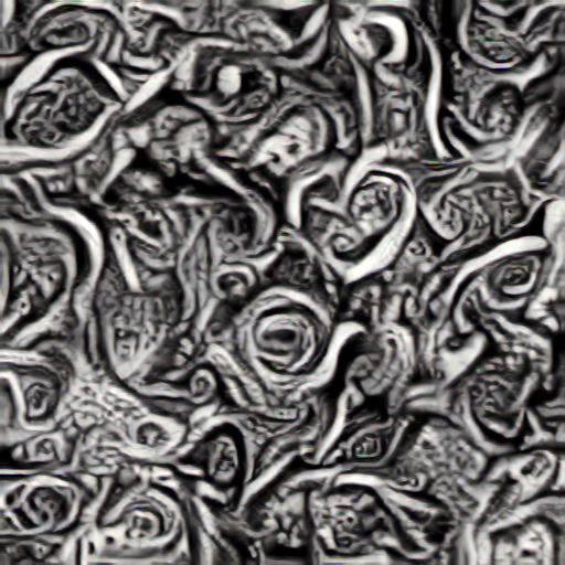
To speed up optimization, we decompose the feature tensors of both images to a set of principal components. These are chosen such that they capture 90% of the total variance in the style features at a given layer depth. These principal components lie along the axes which most contribute to a style’s “character” and so it is sufficient to focus only on optimizing these most important directions. Despite reducing the dimensionality of the features significantly, the effect on quality is minimal as can be seen in the figure below.

The efficiency gains are substantial, however.
Multi-scale synthesis
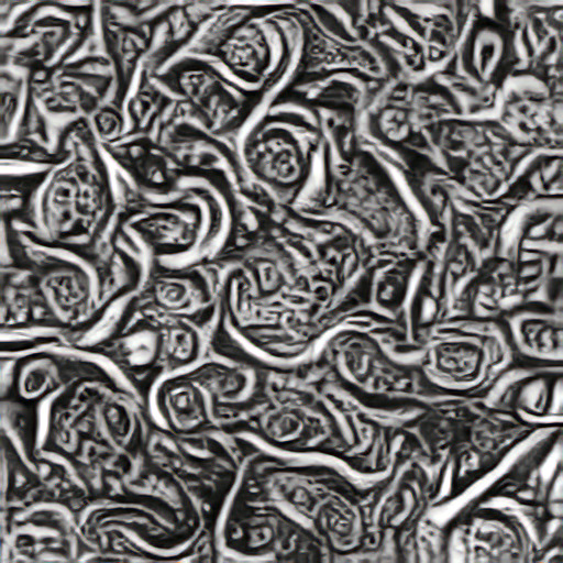
The next performance optimization is multi-scale synthesis. For this we opted to simply upscale the image between each pass of the optimization. The general idea is that at smaller sizes, larger-scale shapes are transfered from the style, while at larger sizes, fine details are transfered.
We linearly space the sizes between 256 pixels and the specified output size. This ensures that details at all scales are captured. We also weight the number of iterations for each size to be greater for smaller (faster) images and less for larger (slower) images. This focuses the optimization on preserving larger-scale aspects of the style and helps improve speed.
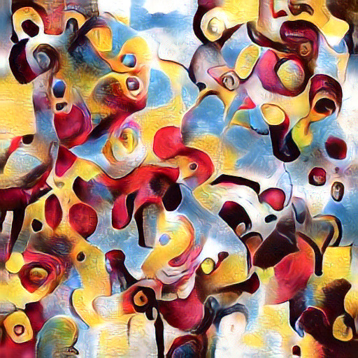
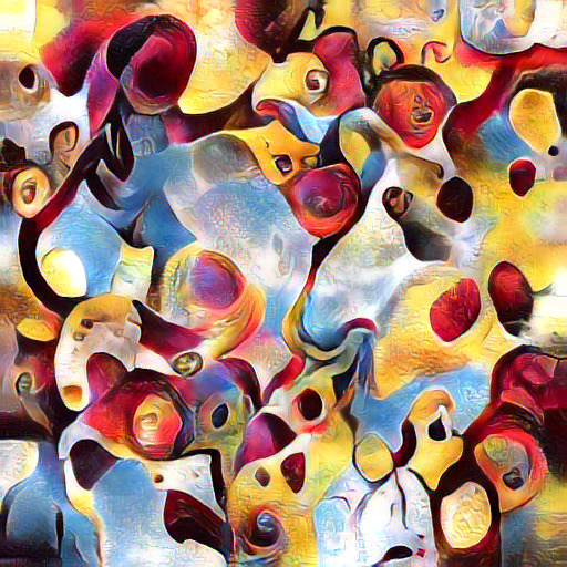
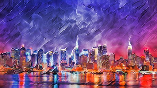
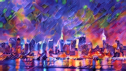
Below we show the effect of multi-scale resolution on output quality. While the trend of preserving larger features is present in our implementation, it is less pronounced than the results of the original paper. We are unsure of the exact cause of this discrepancy, but suspect that the exact number of passes and iterations and sizes optimized at play an important role. These were not specified completely in the paper.

Style transfer
Style transfer is a simple extension of the texture synthesis task. The output image and style image are optimized in the exact same fashion. The content image is also encoded with the VGG network, then its mean is subtracted and that of the style images features added. This ensures that the features of the content and style aren’t competing with each other in terms of any global bias in their feature tensors. Finally, the content is also projected onto the style’s principle component basis.
Rather than matching the histograms of the content and output image, output feature tensor is directly blended with the content’s features at the deepest 3 layers (relu3_1, relu4_1, and relu5_1) after each histogram matching step.


Color transfer
We noticed some discrepancies between our results with optimal color transfer versus those reported in the paper. Shown below is our attempt at recreation of figure 9 from the paper compared with the actual figure.
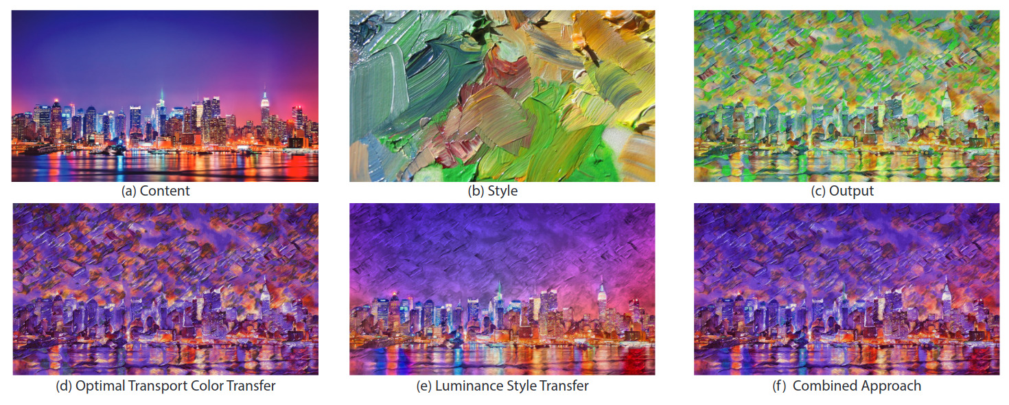
We’re unsure what causes the issue we see, but the added green coloration differs significantly from the expected result. One possible explanation is that our increased number bins in the histogram happens to carry over more green from the histogram of the original content. There is a tiny green spot in the content (bottom right), so the result might just be the algorithm working as intended.
Texture mixing
Our texture mixing results very closely match the results in the paper. The interpolation between the two textures seems semantically smooth.

Our implementation also allows for doing style transfer with mixed textures.
Performance analysis
While the paper reports significantly improved speed relative to the original “A Neural Algorithm of Artistic Style” and improved quality relative to “Universal Style Transfer via Feature Trasforms”, there are other implementations of techniques that are significantly faster or higher quality. To get a sense of how Optimal Textures compares to more recent techniques, we compare it in terms of speed and quality with maua-style and texture-synthesis.
maua-style is my own implementation of the optimization based style transfer approach. It uses multi-scale rendering and histogram matching between each scale, as well as switching to progressively less memory-intensive image recognition networks as the image size increases. These improvements make it faster and higher quality, as well as allowing for much larger images for the same amount of VRAM than the original neural-style.
texture-synthesis is a “non-parametric example-based algorithm for image generation”, in the words of Embark Studios, the company that created the implementation. It progressively fills in the image by using patch level statistics to guess what the value of a pixel should be based on the neighbors that are already present. This results in copies of different parts of the image scattered around the output, yet blending together seamlessly.
Below are the results of running texture synthesis with each of the algorithms for square images of size 256, 512, 724, 1024, 1448, 2048, 2560, and 3072 pixels per side. These results were recorded on a GTX 1080 Ti GPU with 11 GB of VRAM.
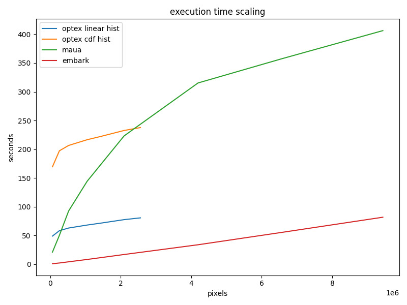
Immediately apparent is the speed and favorable scaling of texture-synthesis (labeled embark). This algorithm scales linearly with the number of pixels in the image. This is logical as it does the same routine for each pixel.
optex is the next fastest algorithm. Although, this is only the case when using the faster linear transform based histogram matching. Even with PCA and multi-scale rendering, the CDF based histogram matching is not able to outperform the multi-scale maua-style. Also notable is that optex ran out of memory for images larger 1448x1448. These OOM errors happened either in the call to torch.svd to calculate PCA of the internal features of relu2_1 or when encoding the image to relu5_1.
Finally, maua-style was able to generate images all the way up to 3072x3072, albeit 8x slower than texture-synthesis and about 3x slower than our optimal textures implementation.
Quality comparison
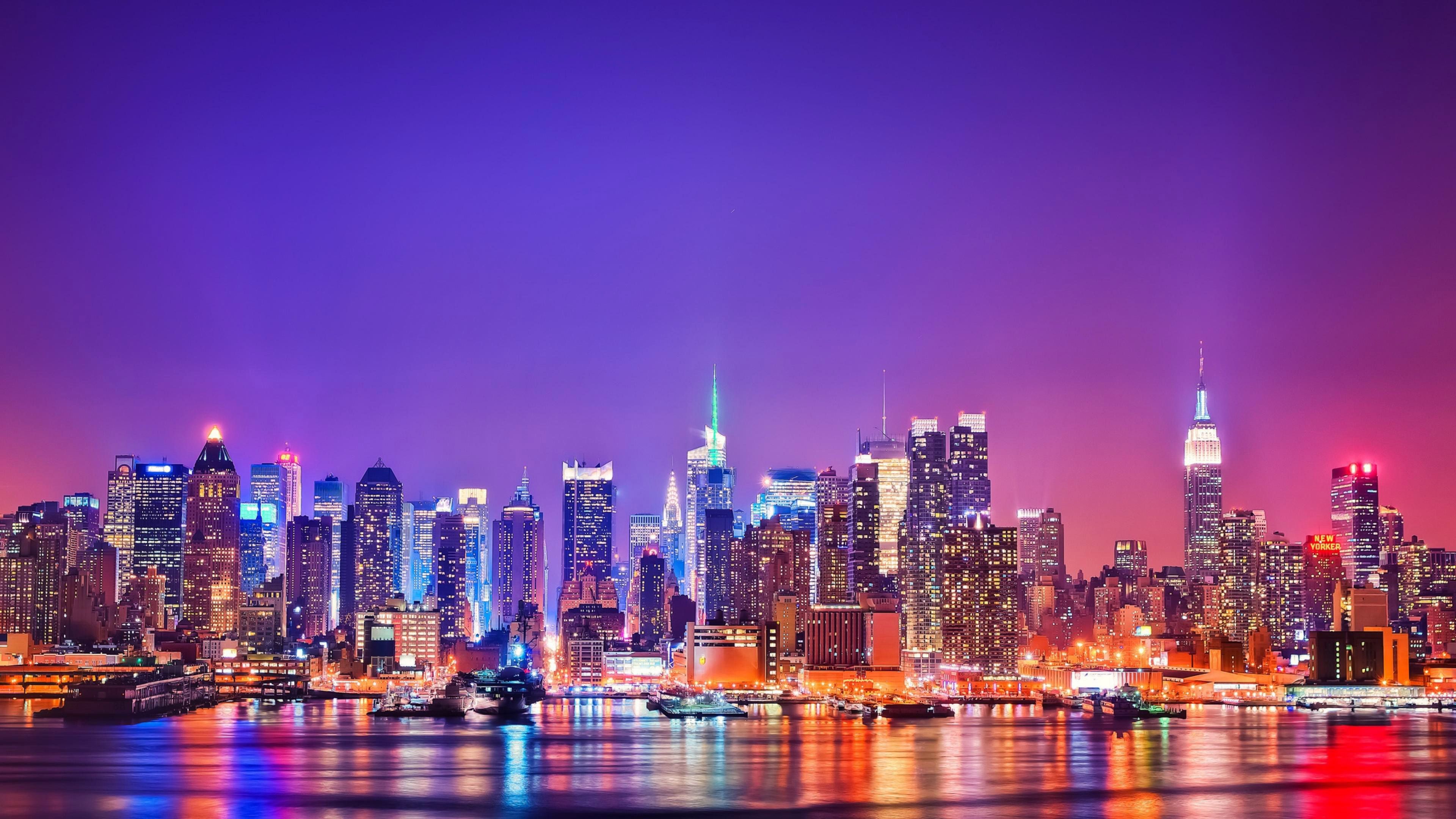
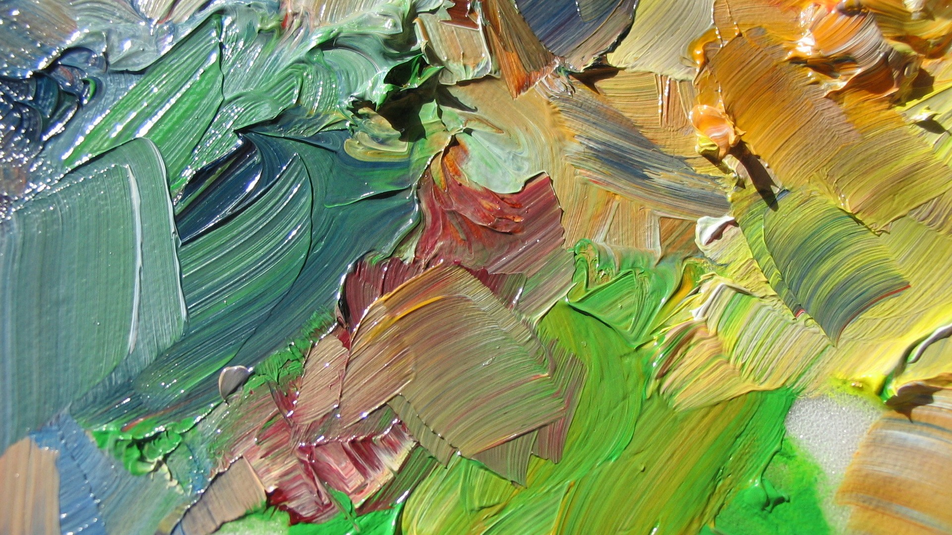
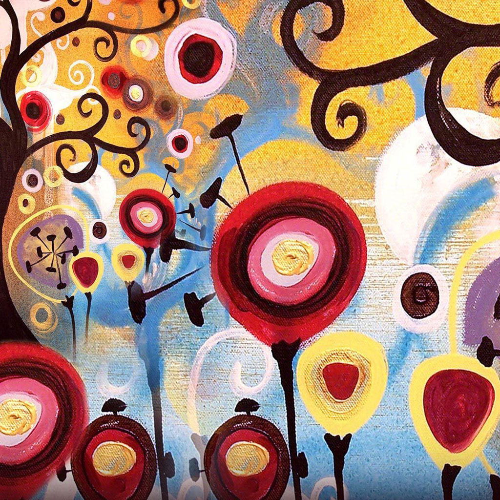
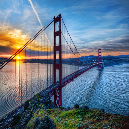
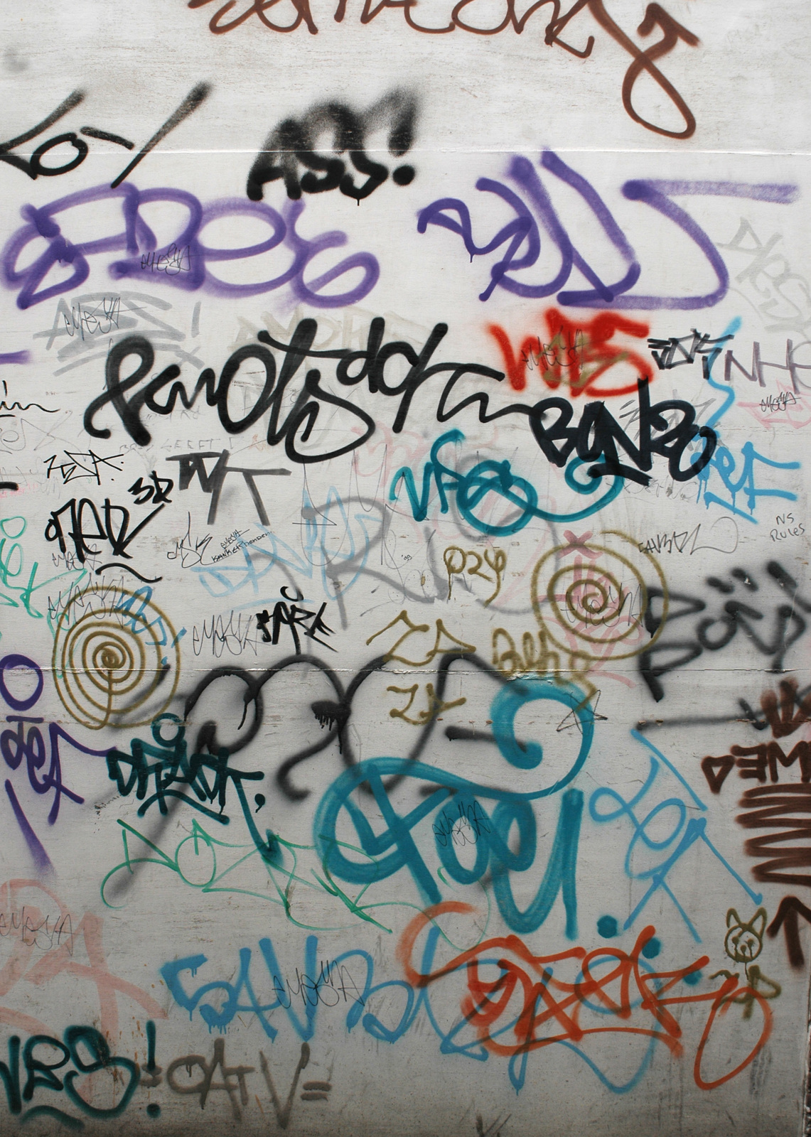
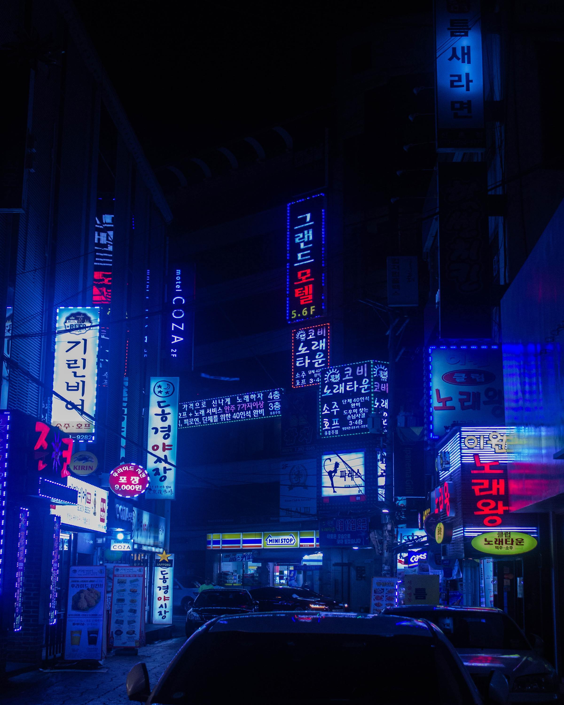
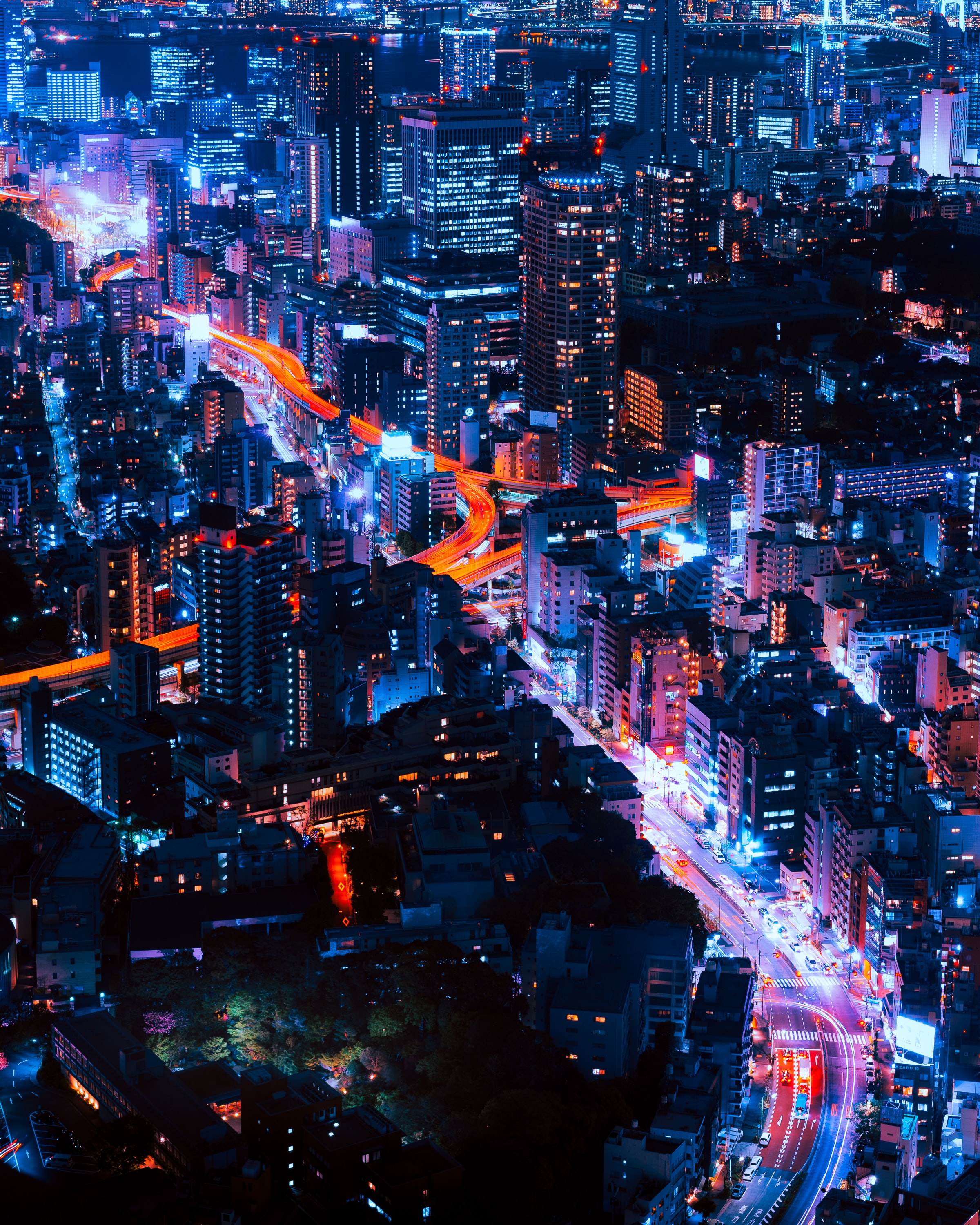
Next we’ll take a look at the quality of results that each algorithm generates. They each have their own distinct character so it might not always be the best choice to just use the fastest one. The input images below are by unsplash.com users Ciaran O’Brien, Pawel Nolbert, V Srinivasan, Franz Schekolin, and Paweł Czerwiński.
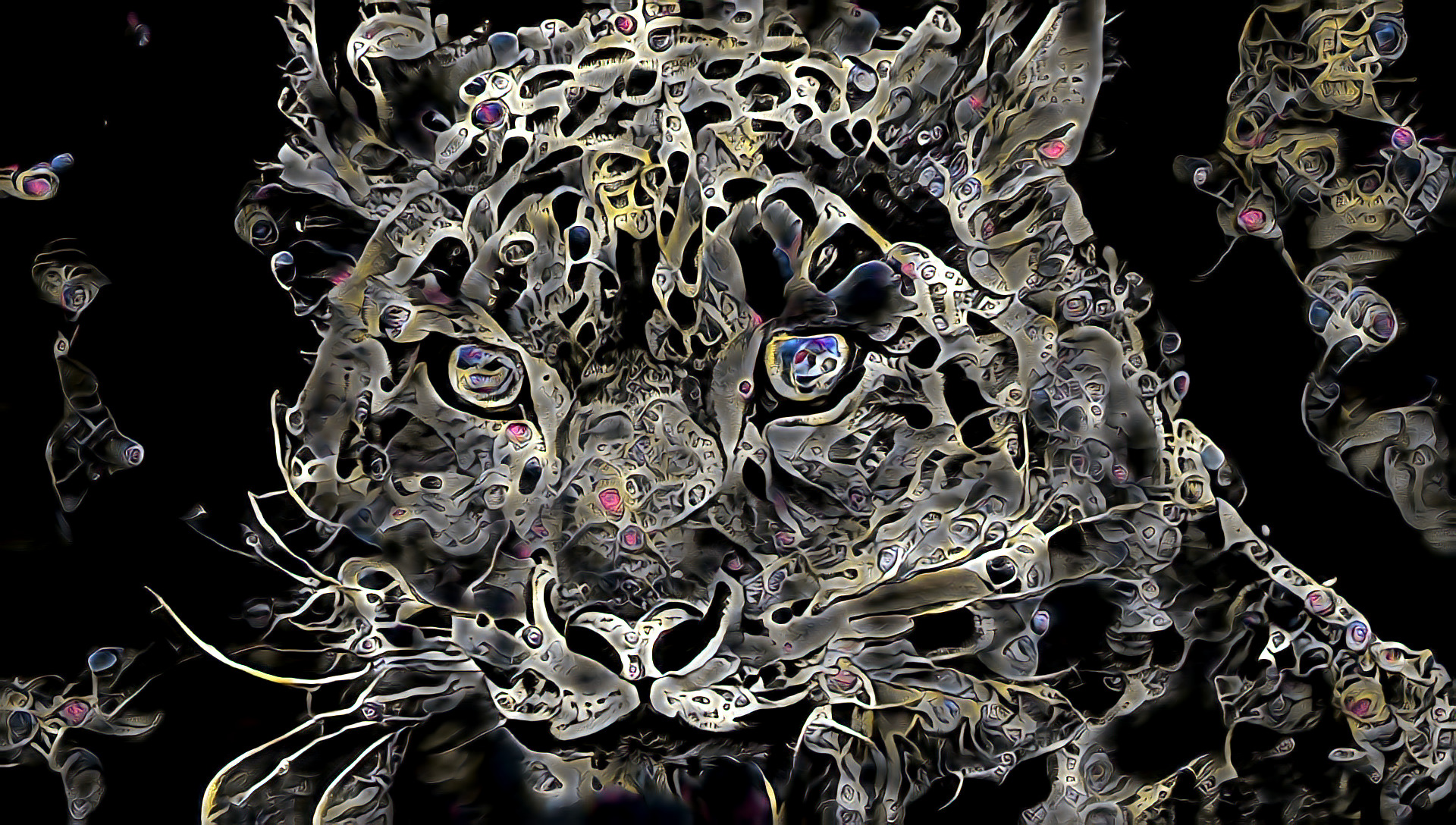
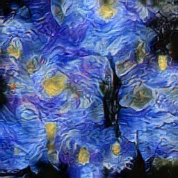
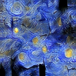
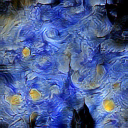
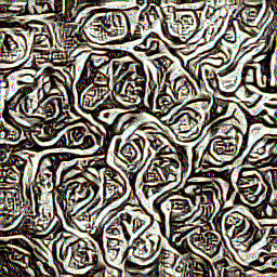
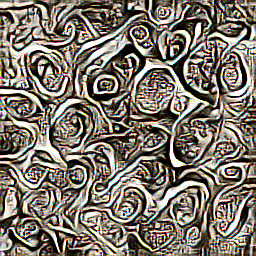
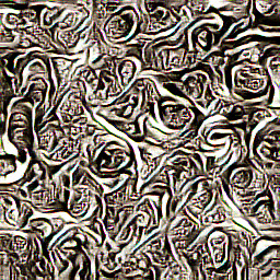
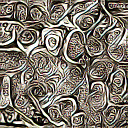
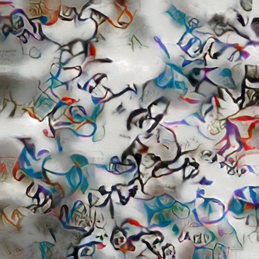
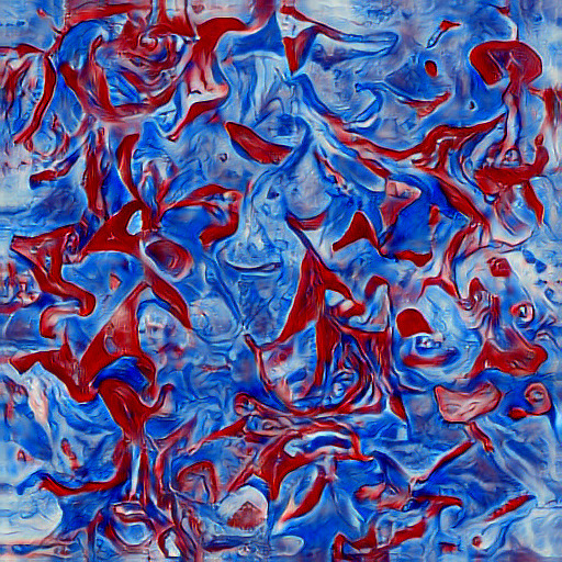
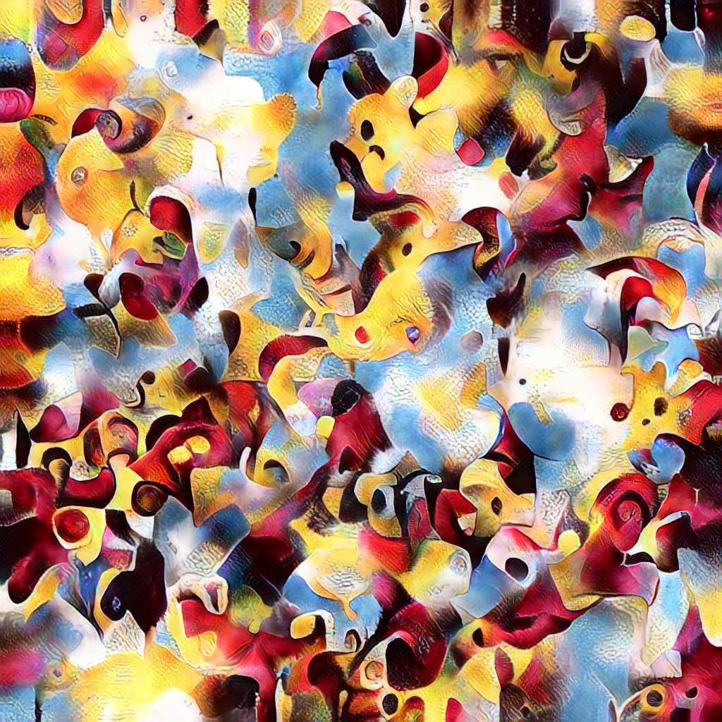
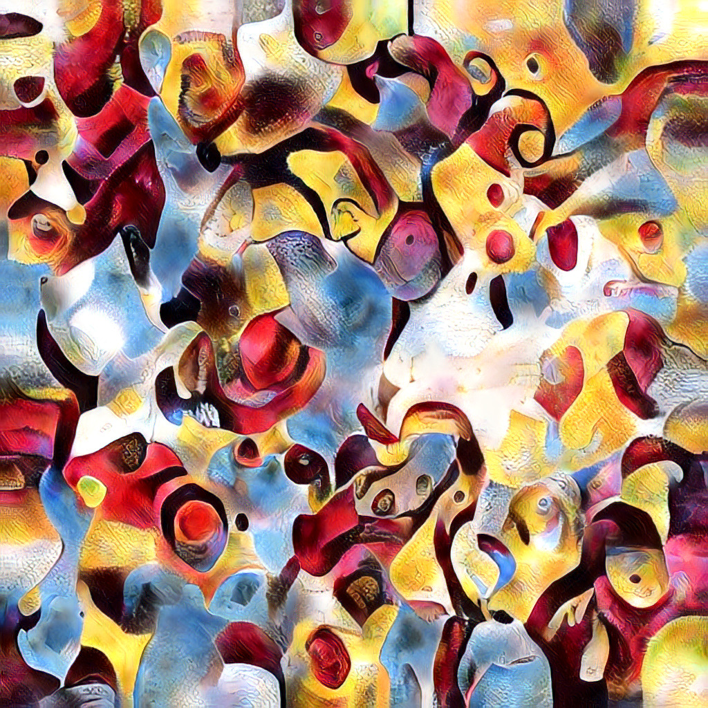
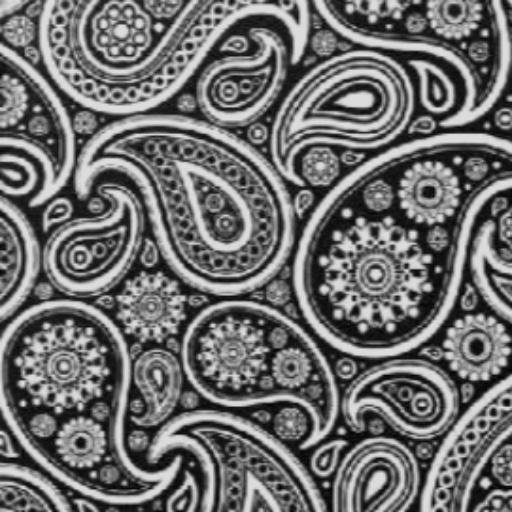
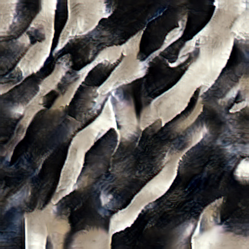
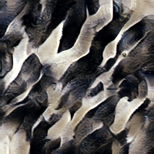
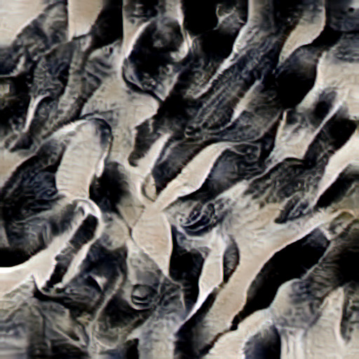
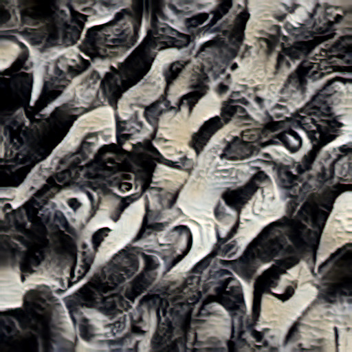
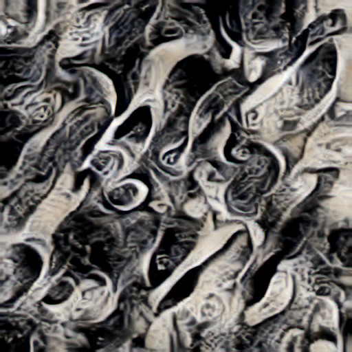
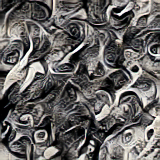
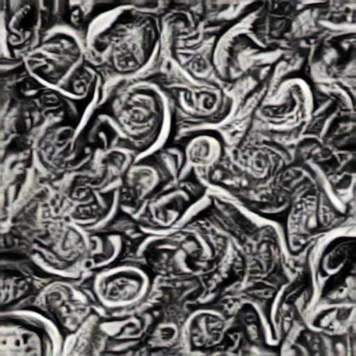
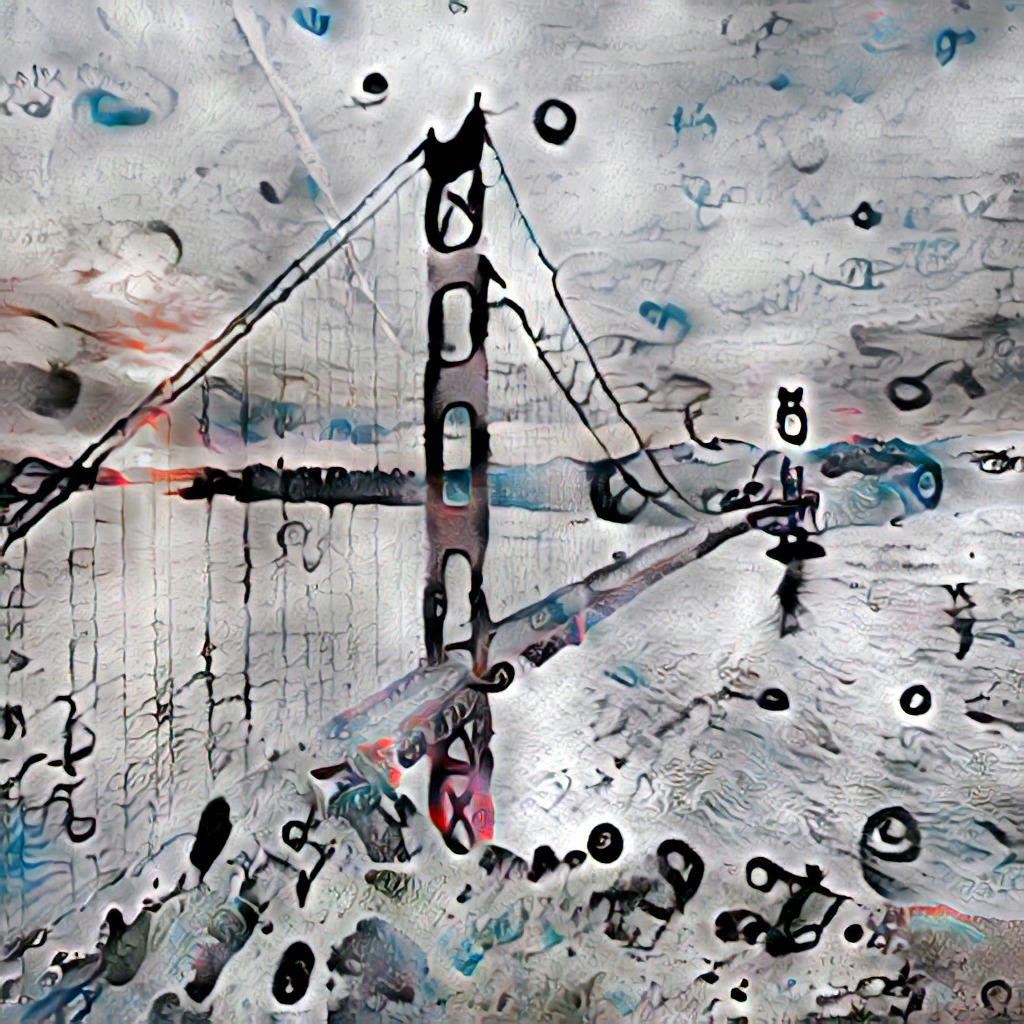
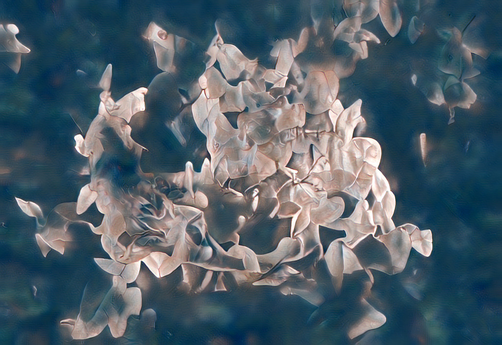
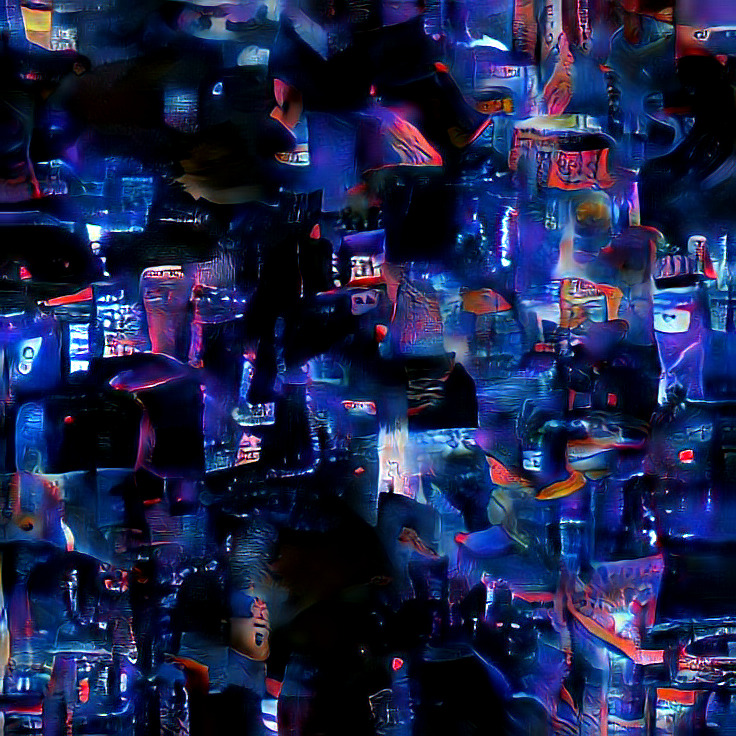
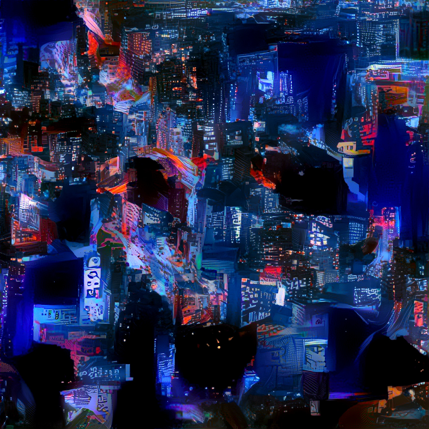
Texture synthesis

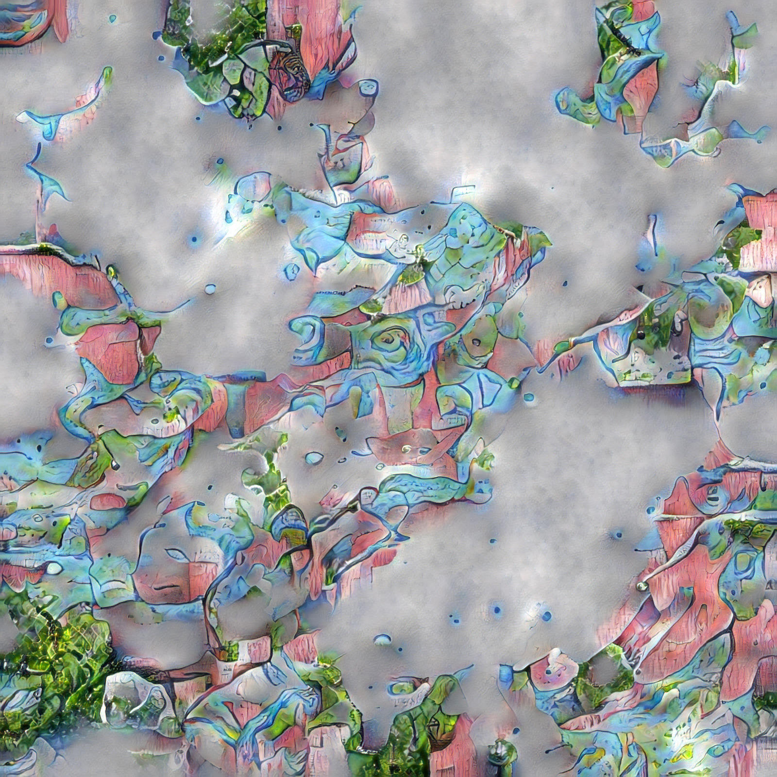
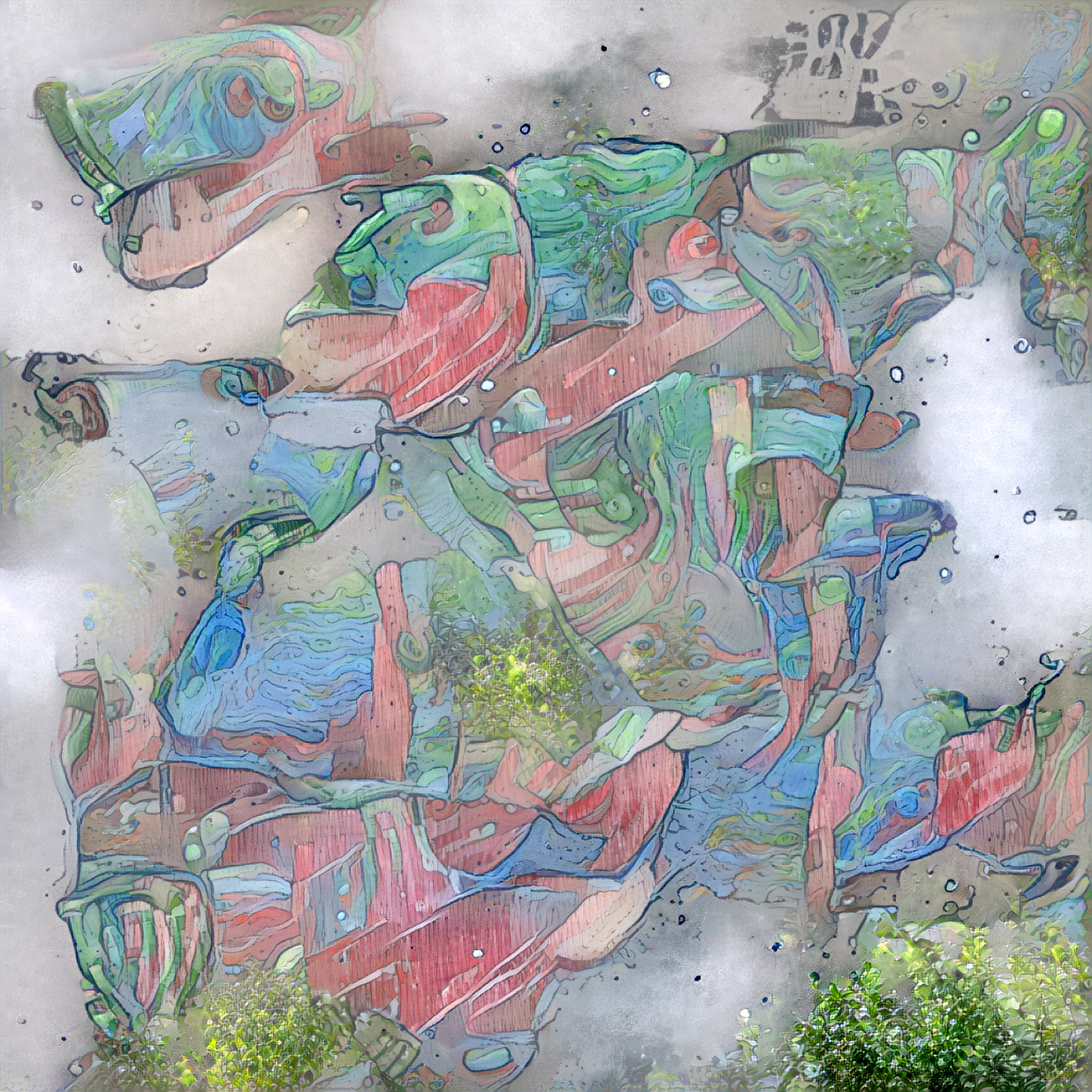
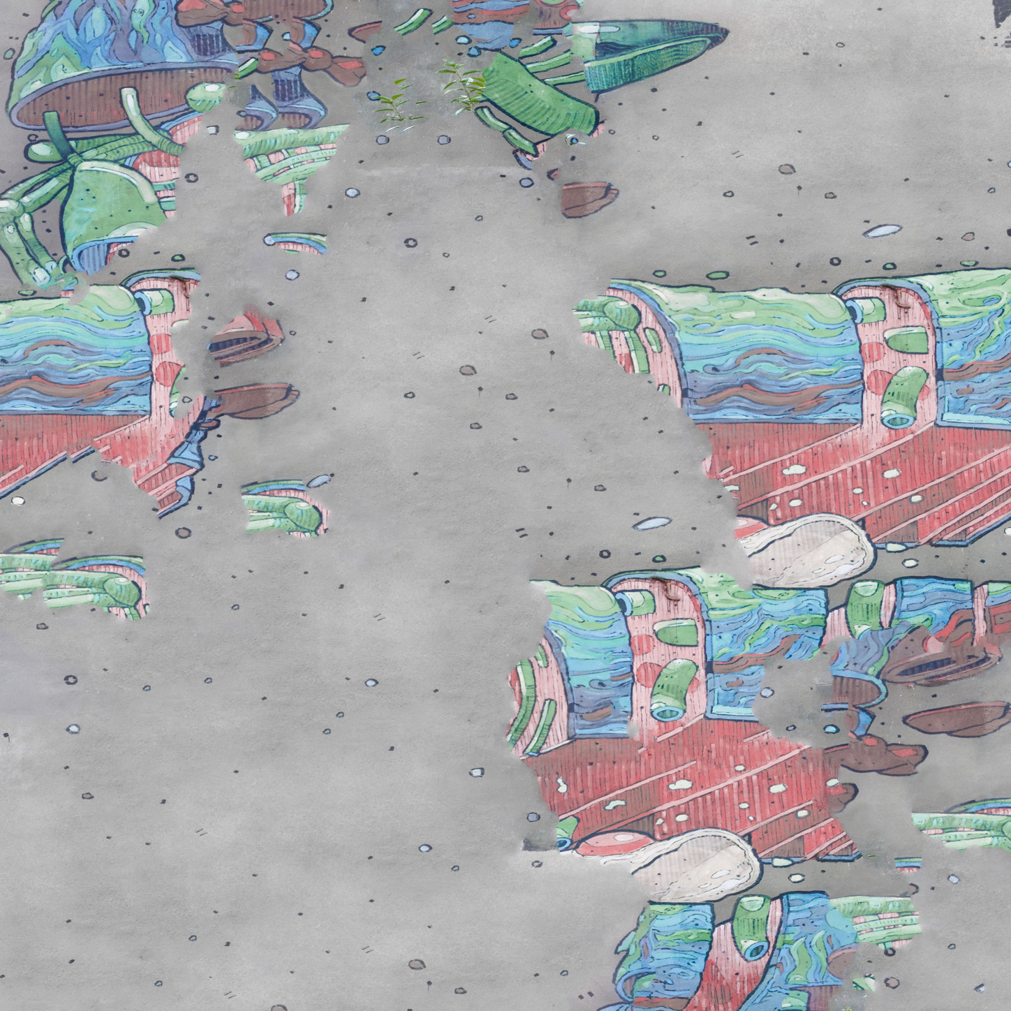
Our optex result seems to be most scrambled of the three approachs. The maua-style result seems to have some faded patches, but reproduces the images characteristics well. The texture-synthesis result is most true to the original texture, there are some duplicate features in the image though.
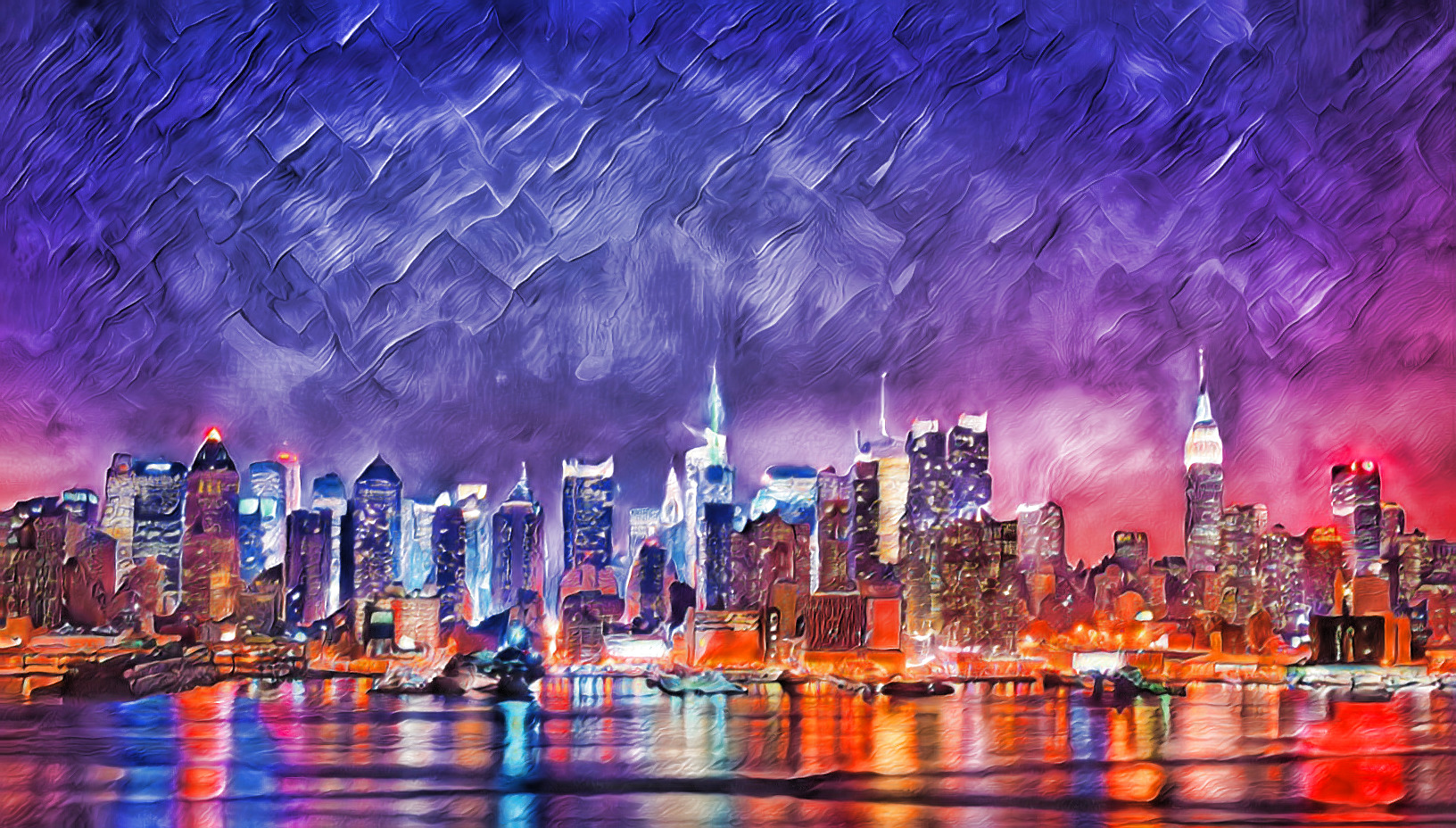
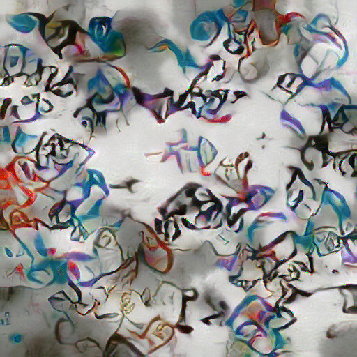
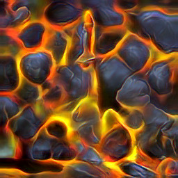
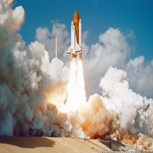
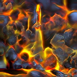
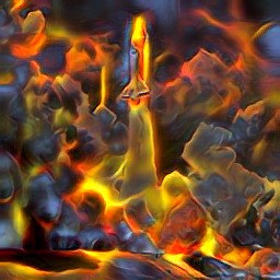
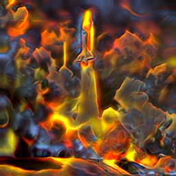
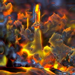
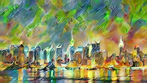
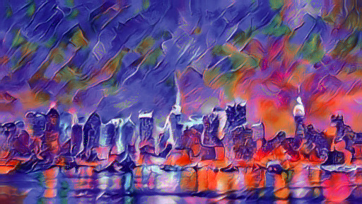
Style transfer
Now for style transfer. The two input images are shown at the top. They are each used as content and style for each other.

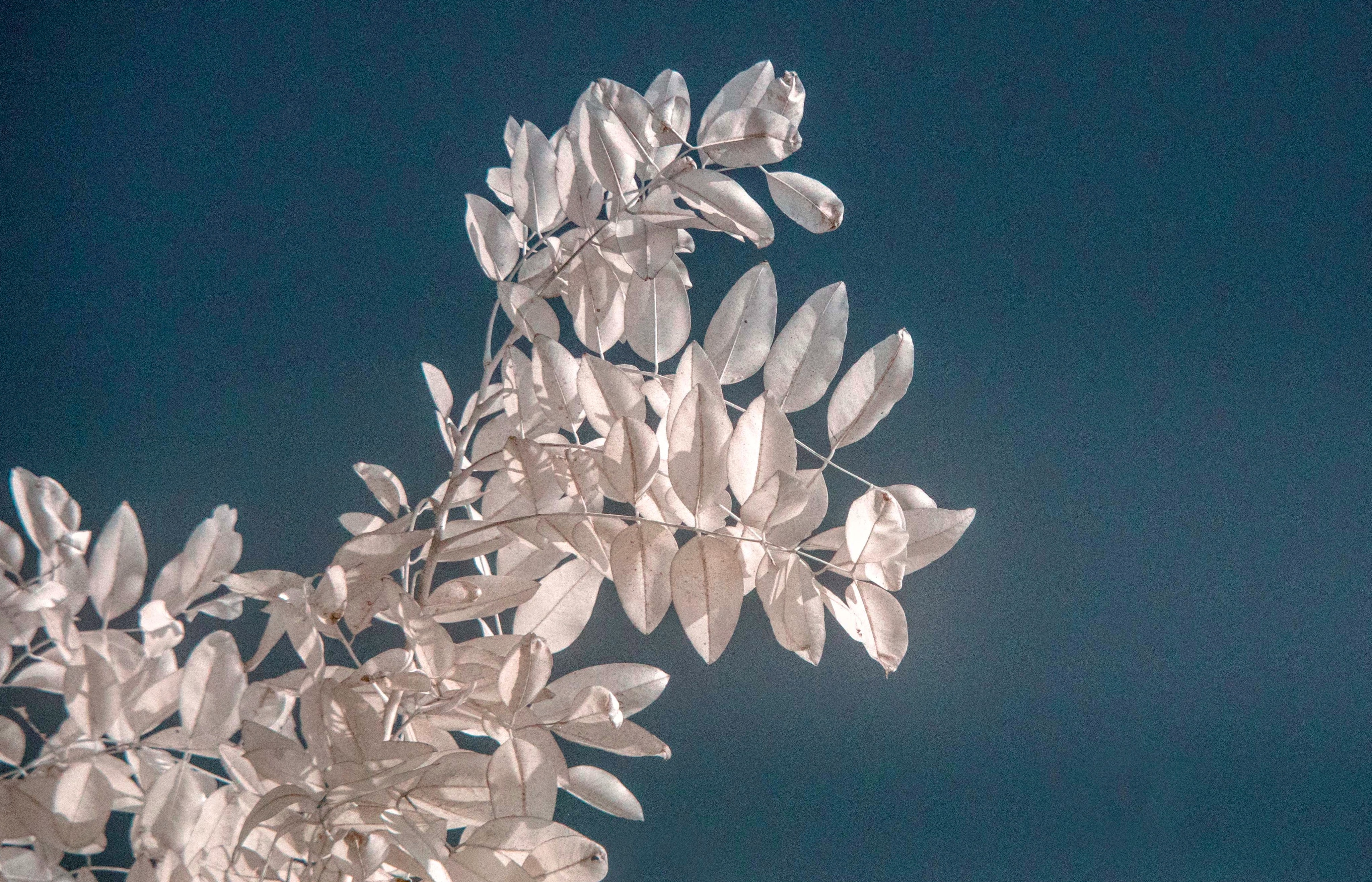
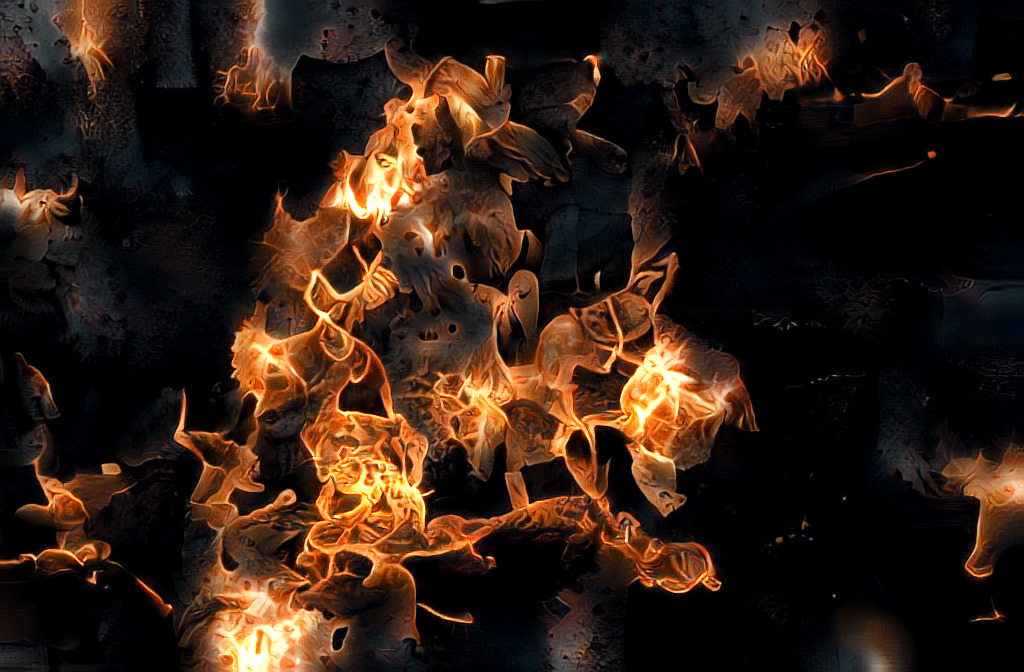
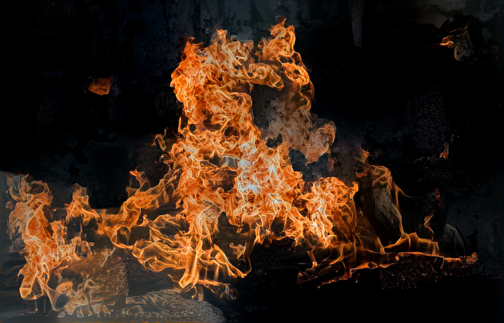

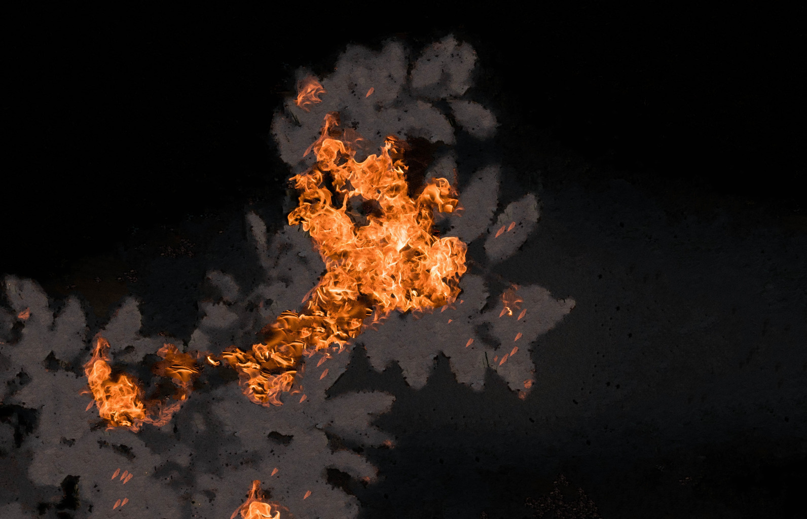
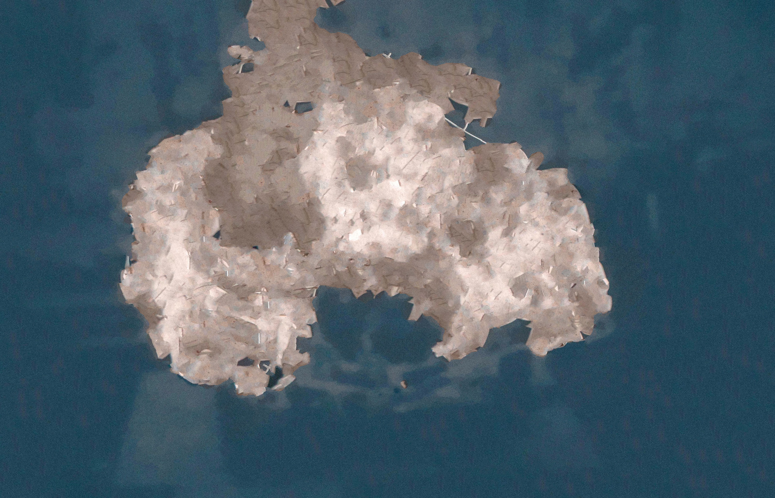
Once again, optex seems to be slightly more scrambled than the other two approaches. The flames/white leaves are all around the image rather than only on the central object. maua-style more faithfully captures the style of each, but has faded patches on the bottom left of the darker image. texture-synthesis seems to overfit to the content in both cases, while not really recreating the style as faithfully. Perhaps the default content-style tradeoff weights the content higher than the other algorithms.
Texture mixing

Here, both optex and maua-style seem to lose most of the larger structure in the images. However, the blend between the styles is fairly good. texture-synthesis is very clearly copying over large parts of the images here. It has essentially just spliced them into the top left and bottom right corners, not really blending successfully.
Final thoughts
All in all, our replication of “Optimal Textures” has been a success. We were able to implement the majority of the techniques discussed in the paper. We built on the pre-trained VGG-19 autoencoder from “Universal Style Transfer via Feature Trasforms”, we made liberal use of code we found online (thank you SciPy, NumPy, and ProGamerGov!), and finally were able to link it all together in pure PyTorch to create a working algorithm.
The method does indeed have a strong speed/quality tradeoff, however, it still leaves room for improvement in terms of larger-scale features of textures. Perhaps a combination of this fast histogram matching with the slower, high-quality optimization approach can bring together the best parts of each algorithm.
We would like to thank the organizers of the course for the great project and Casper van Engelenburg for his guidance and feedback along the way. If you made it all the way the way through this, thank you for reading, and feel free to give optex a try yourself!