Lakspe is a dataset I made with an eye on StyleGAN1–my first foray into the latest and greatest generative model at the time. StyleGAN works best when there is a uniform structural similarity in the images it’s trained on (e.g. centered faces or sketches of beetles2). The more similar the images, the better StyleGAN will reproduce them and the more varied the details will be. Training with more varied sets works too3, but I wanted to play to StyleGAN’s strengths to start off.
I set out with a goal of making animations that were full HD (1920x1080 resolution). I knew I wouldn’t be able to train at that resolution (and at the time I didn’t know that the fully-convolutional StyleGAN generator could just generate larger images than it was trained on at inference time), so I decided I could hack my way to a larger resolution by making sure that the edges of my images were all the same color. That way I could just pad my frames out to the resolution I wanted. This also opened the door to fun things like multiple objects moving around on one larger canvas while interpolating individually.
However, there was one big problem, how could I ensure the edges of my dataset were all the same color? I was planning to generate my dataset using recombinant style transfer4, but one of the major drawbacks of style transfer is that taking the gram matrix of internal features of a neural network discards long-range spatial correlations–smearing the styles out all over the image. This can be offset a little by ensuring the content and style images all have one color around the edges, but that puts a lot of constraints on which images can be used. Even still, convolutions can cause artifacts around the edges which are brought out by subsequent passes at higher resolutions. What I’ve often done for one-off images is to just clean up the edges manually once I’m happy with the rest of the image, but that clearly wasn’t going to scale well for the thousands of images I would need to train a GAN. I needed a better approach.
Before I explain how I cleaned up the images, let’s take a look at what I was working with…
Style Transfer
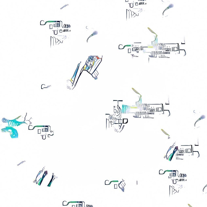
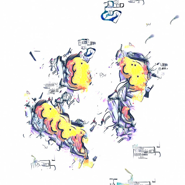
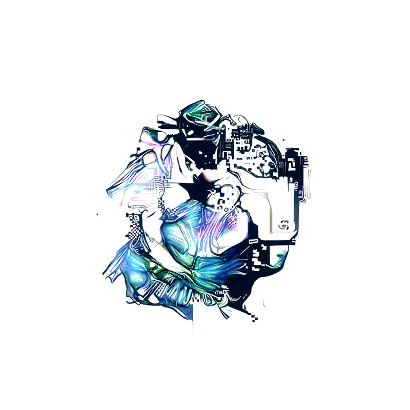
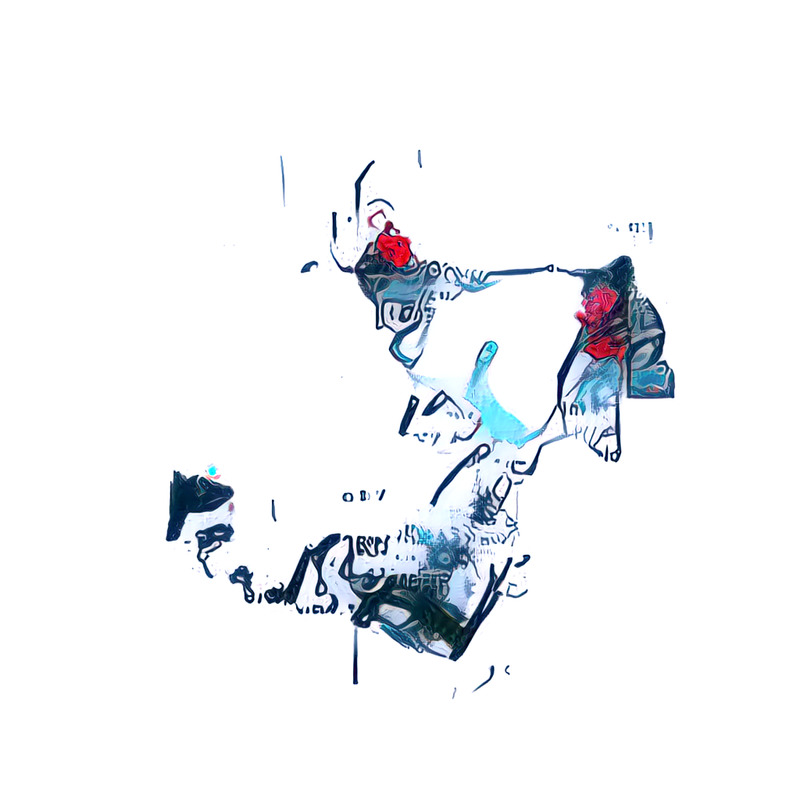
To start off, I went through my big ol’ folder of images and selected about 20-30 colorful, high-contrast images with a white background. I reverse image searched some of them and grabbed a bunch more images from the “visually similar” results. Then, with 70 style images and about 20 content images with simple, centered objects, I started the first round of style transfers. Each time selecting 1-3 images randomly as styles.
Texture Synthesis
While my GPUs were hard at work generating images for me, I stumbled across Embark Studios’ just-released texture-synthesis5. Not only was it flexible–allowing for synthesis, style transfer, in-painting, tiling, and more–but it was also CPU-based and fast. At first it was taking 5-10 minutes to generate images slightly smaller than my style transfers (when using 1-3 inputs of 2-4 megapixels). However, I saw there was a pull request6 open from someone who had found that the majority of time was spent in a loop that could be memoized. With this small patch applied, the time to generate images at my target resolution dropped to only 30 seconds! This meant I could use my CPU to generate images alongside my GPUs and it would be generating 4 times as many images per minute.
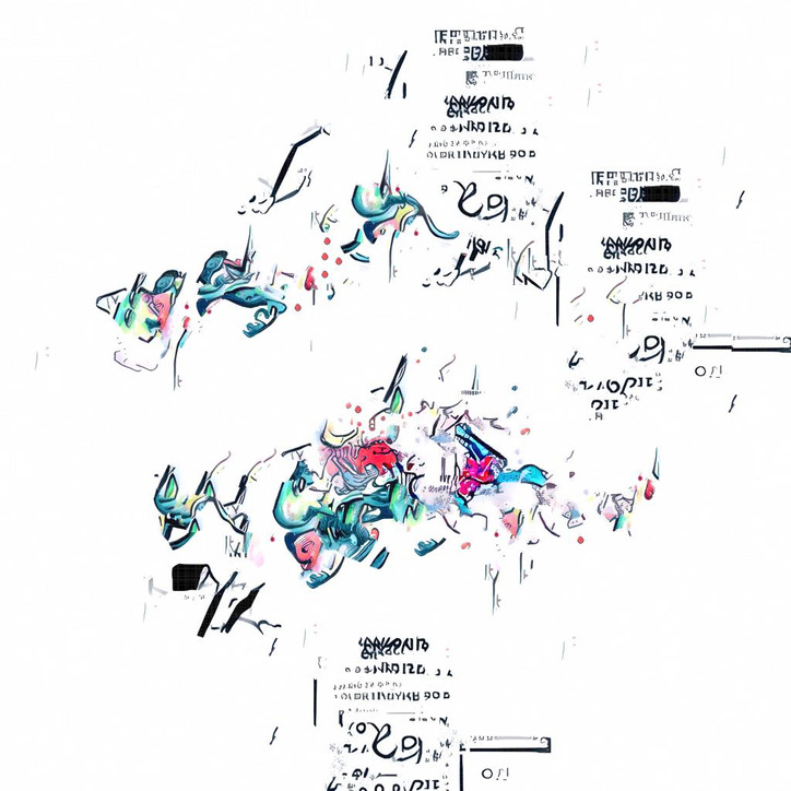
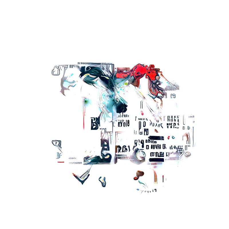
In a nutshell, the most basic form of the texture synthesis algorithm works by looking at all 9x9 patches of the input images. It then chooses a random pixel in the generated image, checks the colors of that pixel’s neighbors, and looks up in the set of patches which color is most likely, based on the already-filled-in neighbors. Of course, searching through every 9x9 patch of an image for every pixel is infeasible for larger images. There’s a couple of crucial tricks that speed up the process and improve the results versus the naive approach.
First off, instead of using 9x9 patches, the k nearest, already-resolved neighbors of each pixel are allowed to “vote” on the value. Their votes are weighted by the distance to the pixel. Another important trick is to progressively deblur the example image as the distance to the nearest, already-resolved neighbors decreases. The idea here is that, early on in generation, the exact pixel values aren’t important, but rather the average color over a larger spatial area is. As more of the image is filled in (and so the average distance to the nearest neighbor pixels is smaller), more small-scale information should be incorporated to refine generation.
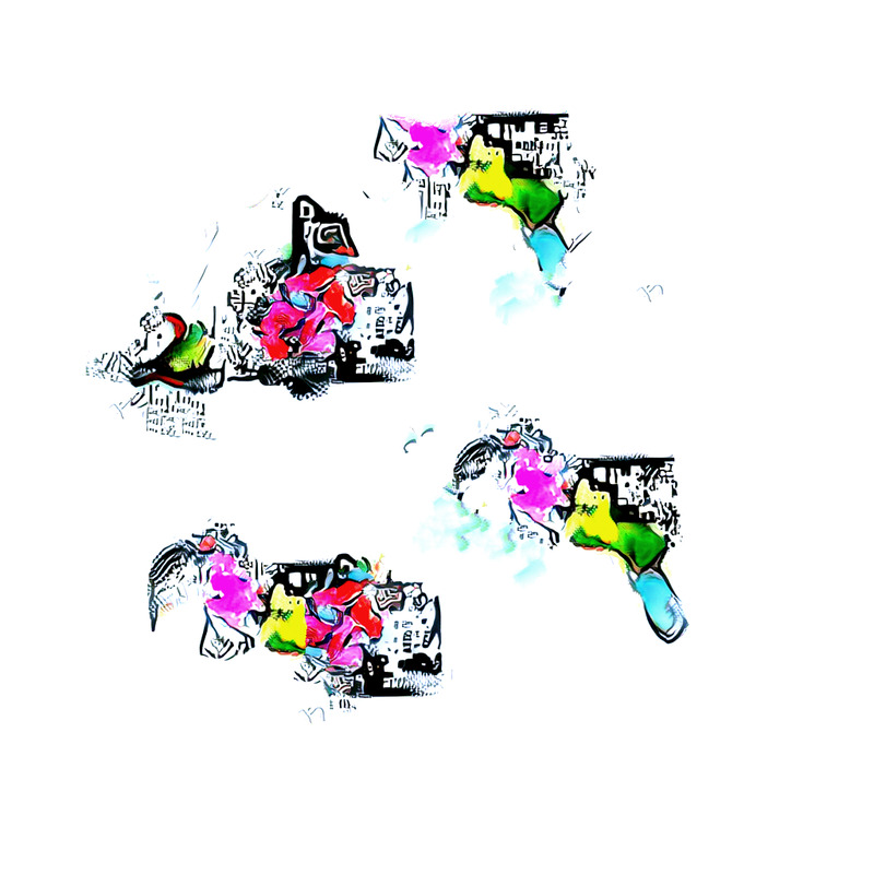
The result is a kind of franken-patchwork of parts from different examples stitched together in a locally-coherent way. I especially love the repeated parts which seem like they’ve been copied, but, on closer inspection, join together to their surroundings in different ways. I also like the little sattelite patterns scattered about–each seeded by a single lucky black pixel.
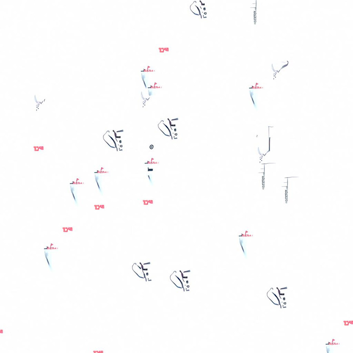
While these texture synthesis results were generally a lot cleaner than the raw style transfer images, there was still too much going on around the edges. Let’s get into how I cleaned ‘em up.
Seam Carving
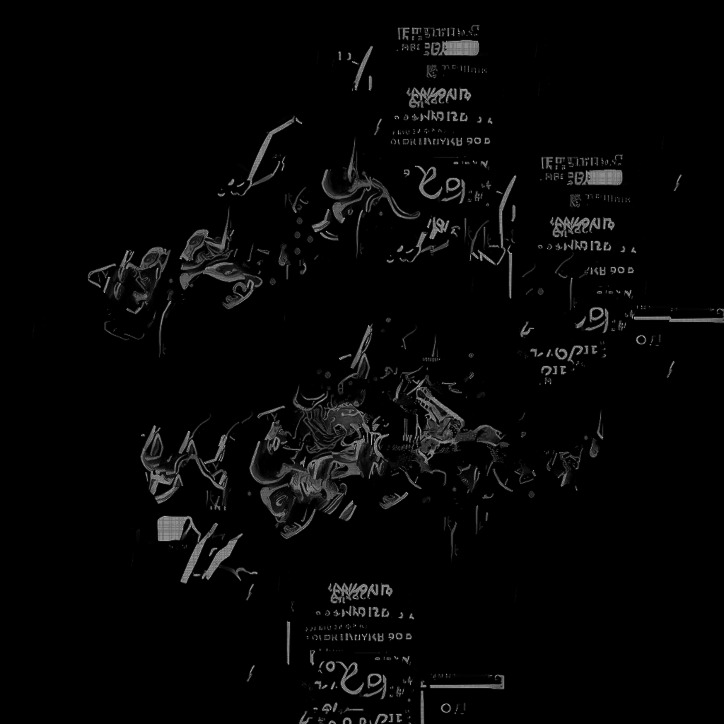
What sparked me to start working on the dataset was a post on seam carving by Avik Das7. The post discusses a way to resize images in a content-aware fashion by removing “seams” of pixels with a “low energy”. A seam is a vertical (or horizontal) string of pixels that differ in each row by maximally one position from their predecessor (i.e. a connected, but probably crooked, line from top to bottom). The energy of a seam (the sum of the energy of its component pixels) can be defined in many ways, but one simple way is by looking at the difference between a pixel and its neighbors. A seam with low energy will be very similar to its neighboring pixels along the entire length, and so removing it will ensure that the newly neighboring pixels are still similar. By repeatedly finding the lowest energy seam and removing it, an image can be resized along an axis by removing only “dispensable” pixels.
Finding the lowest energy seams also has a simple dynamic programming solution which makes the whole process pretty efficient. Iterate over the rows of the image and for each pixel note which of its three neighbors in the previous row has the lowest energy. Set the energy of the current pixel to the sum of the best previous seam energy and the energy of the pixel itself. In the final row, the minimum-energy pixel is the tail of the lowest energy seam.
While I was reading, the idea came to me that maybe I could use a similar approach to clean up the edges of my images. I could find a seam around the center of the image with low energy (i.e. that didn’t cut through any of the cool things the style transfer / texture synthesis had generated) and then set all the pixels outside that seam to my background color. There was a little bit of a problem though. The dynamic program relies on memoizing the best seam up to the 3 possible predecessors of a given pixel. However, in the case of a circular seam, it’s unclear exactly which pixels need to be considered. The possible predecessors vary based on where in the image the pixel is. If we assume the seam goes clockwise around the center of the image, on the left side of the image, pixels below the current pixel should be considered, while at the top of the image, it should be the left neighbors.
At first I was thinking of adding helper functions that would return the coordinates of the possible predecessors, but this would still require a complicated iteration scheme to ensure that previous neighbors had always already been processed. This would work if I were to repeatedly iterate over the radii to the edge of the image. Then the previous “row” would be the pixels in the previous radius.
💡
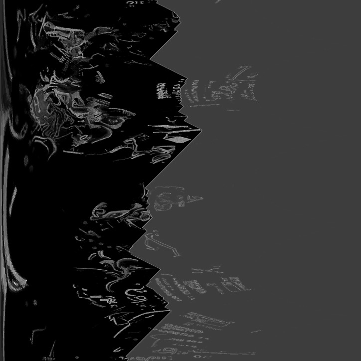
Instead of all this radius-based iterating and mapping between coordinates, I could just transform my energy matrix to polar coordinates so that each row was the pixels along a radius at a different angle! This way, I could just apply the regular seam finding algorithm to the transformed matrix without all the weird hacks and helpers.
This gave the following algorithm: calculate the energy of all the pixels in the image, warp the energy image to polar coordinates, find the lowest energy seam with the dynamic program, fill the area right of the seam with background color, and warp back to regular coordinates.
Tweaks & Improvements
While this algorithm is pretty decent, it doesn’t deliver the best results without some finetuning.
First of all, warping an image to and from polar space isn’t lossless and causes a lot of pixelization (at least with the OpenCV implementation I used). So rather than painting over the original in polar space and transforming back, it’s better to use a mask. Transforming the mask still pixelates it along the edges, but a little gaussian blur smooths this out and creates a nice fade for places where the seam ends up cutting through objects.
Secondly, the dynamic program is pretty ruthless in its search for the lowest energy seam, which leads to some less-than-ideal results.
Although, the seam will sometimes need to go through objects, I wanted to avoid that as much as possible. The “difference with neighbors” energy function tends to have high values along edges, but not inside a given area of the same color. This means that seams only needs to cross two high-energy lines and so often still end up cutting through objects. To discourage this, I adjusted the energy function to also have a term for the difference between the pixel value and the background color. This explicitly biased the seams to only cut through the white background in my images.
Another problem is that when the energy image is warped to polar coordinates, some pixels from outside the original image are warped into the transformed image. This happens because the the distance to the corners of a rectangular image is larger than the distance to the edges. To ensure all pixels from the original image are in the polar coordinate image, all coordinates in the circle that circumscribes the image are considered. This means a bunch of pixels from outside the original image are mapped into the new image. These pixels have 0 energy and so the optimal seam just cuts around the outside, only touching the corner pixels. This is easily alleviated by filling pixels that are mapped from outside the original image with high energy values.
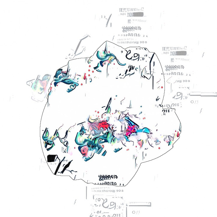
With that exploit taken care of, the dynamic program finds another shortcut. When there happens to be nothing in the center of the image, there’s a nice, low-energy seam which stays at radius zero through all angles–leaving a blank image behind. I wanted as much object in my images as possible, while still leaving the corners free. To encourage this, I added extra energy to the center of the image that scaled down quadratically to 0 at half the radius. This made sure that the central objects were pretty big, but that the seam could still cut inside a little if that allowed a substantially lower energy seam.
The last problem I needed to pin down I dubbed the snailshell problem. Sometimes the most optimal seam started at a radius different from where it ended. This created masks that looked kind of like snailshells–an outward spiral, sealed shut. Usually this wasn’t an issue, but in some unlucky cases this resulted in a nasty straight cut in the cleaned image.
It took me a while to think of a way to solve this, but in the end the solution was quite simple. Once the dynamic program had calculated the energy up to the last pixels, rather than selecting the minimum seam immediately, the energy of the pixels in the final row with radii between the seam’s head and tail were added to the energy. This explicitly accounted for the pixels that the seam would be cutting through if it was a snailshell. All that was needed was a little bit of extra bookkeeping to record the x-coordinate of the head of each seam.
With these changes the algorithm produced nice results on all the images I checked. While it wasn’t the fastest implementation, being in python, the 7 seconds required per image was pretty much negligble compared to the 3-4 minutes required for each style transfer.
Results
Once I had a couple hundred images cleaned up, I started feeding images back into the style transfer and texture synthesis loops. I slowly made the chance of selecting from the original style and content images go to zero while boosting the chance of some of my favorites up ‘til then. In the end, the raw dataset was about 4000 strong. Before letting StyleGAN loose on it, I augmented that up to about 20000 using Albumentations8–adding affine shifts, zooms, flips, rotations, and hue shifts to increase variety.
After a good 2.5 weeks of training on two 1080Tis, I was pretty happy with the results. I’ll leave you with this interpolation video as this post is long enough as it is, but rest assured I have a lot more plans for this particular network! I hope this post gives some insight into how I approach things and inspires you to get creative with the datasets you train on. Thanks for reading :)
Footnotes
1 StyleGAN [paper], StyleGAN2 [paper], and my own repository with code for many of my experiments [code]
2 Confusing Coleopterists: Breeding Bugs in the Latent Space [blog]
3 Cyphept: Training StyleGANs on High Variance Datasets [Coming soon…]
4 I’ve covered my recombinant style transfer strategy in-depth in my post on Rhodops [blog]
5 Embark Studios’ texture-synthesis [code]
6 Long live Austin Jones! [pull request]
7 Real-world Dynamic Programming: Seam Carving [blog]
8 Albumentations: fast and flexible image augmentations [code]